Continuity · Grasshopper 2 Docs

Continuity

When talking about the shape of objects, terms like “smooth”, “jagged”, “polished” and “flush” are commonly used and everyone knows what those words refer to. Yet it is difficult to be rigorous with this vocabulary. Is a heron egg smoother than a chicken egg? Are the corners on an iPhone smoother than those on a Samsung Galaxy? The mathematics of continuity provides a quantitative way to measure, compare and discuss these properties.

The concept of geometric continuity borrows heavily from calculus and analysis on a theoretical level, but allows for an easier intuitive understanding, as well as a more immediate translation into real-world issues. We shall postpone discussing the underlying mathematics until the final section of this topic. The first section will introduce the terminology required for any informed discussion involving continuity.

Note that curvature is a related, but different topic. It is nearly impossible to speak of either curvature or continuity without mentioning the other, yet these properties can vary independently and rely on different mathematics.

Geometric Continuity

Continuity is a measure of the smoothness of a shape, either at a specific point, or for the shape as a whole. It is an important property and can have a big impact on the visual quality, the material strength and the fabrication process of a product. A firm grasp of this topic is therefore a prerequisite for anyone engaged in product design or manufacture.

Shapes and transitions across shapes are grouped in discrete continuity classes usually labeled Gₙ or Cₙ, where the subscript is an integer indicating the degree of continuity. The first few degrees are associated with ordinary words correlating to intuitive concepts, but higher ones are too abstract to be easily named using everyday language. Luckily, the lowest degrees are by far the most common ones.

Curve Continuity

The simplest case of continuity applies to two-dimensional curve geometry. Many fringe complications that occur in higher dimensions or with surfaces can be avoided by limiting ourselves to planar curves.

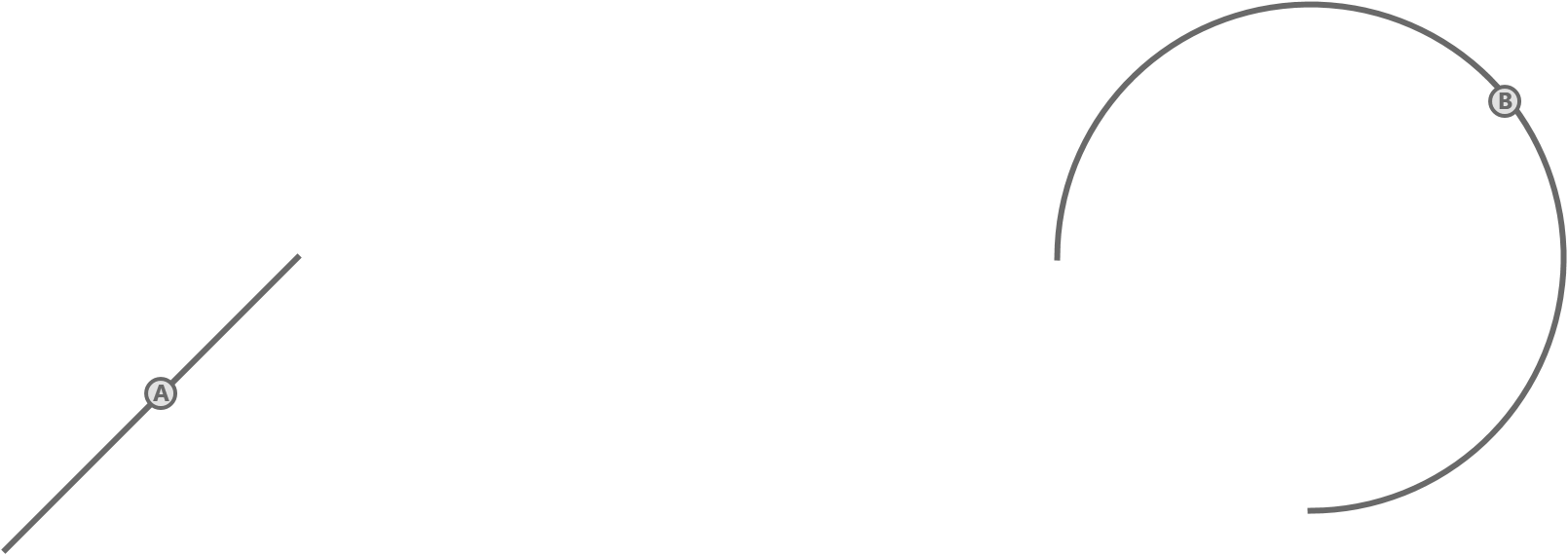
We will start by positing a completely discontinuous geometric set up consisting of two curves in the plane; a linear segment A and a circular segment B, as shown in Figure 1. By inserting a connecting segment C into this set up, we can create a single curve without gaps, whose continuity will depend on the smoothness of this connection.

Figure 1. Two entirely discontinuous curves.

In order to achieve the lowest level of continuity we can connect the ends of the two segments with a straight line, as per Figure 2. This yields a single curve with two kinks in its interior where the new segment C joins with the pre-existing segments A and B.

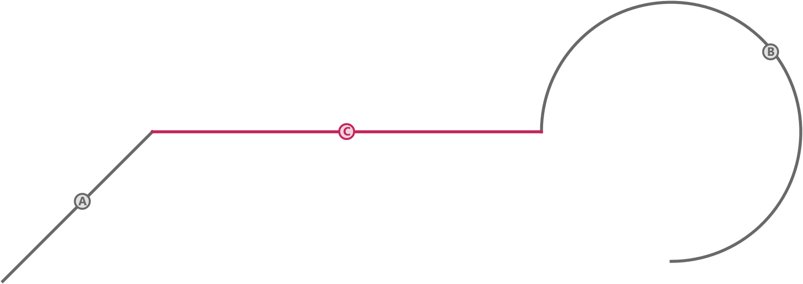
Figure 2. A position-continuous curve can be made simply by connecting all disjointed segments with straight lines.

The continuity at these kinks —and by extension the continuity of the curve as a whole— is called $G_{0}$ , which is the lowest possible degree. In regular parlance this is called positional continuity.

The problem with positional continuity is that it is blatantly obvious that the shape consists of multiple segments. This may be a desired aspect of a design, but more often than not it looks unintentional. Especially in computer graphics $G_{0}$ continuity will make the result appear digital rather than realistic. Furthermore, it can be very difficult to manufacture and dangerous to distribute objects with sharp corners and edges.

Even those consumer products which appear to have sharp kinks from afar will in fact contain higher continuity blending when examined up close.

Kinks can be avoided by joining the A and B segments with a $G_{1}$ , or tangency continuous connection. This degree of continuity requires that the connecting segment C satisfy four constraints; two positional constraints inherited from $G_{0}$ continuity (1 and 2), and two additional tangent constraints (3 and 4):

The start of C must be coincident with the end of A.
The end of C must be coincident with the start of B.
The start of C must be parallel with the end of A.
The end of C must be parallel with the start of B.

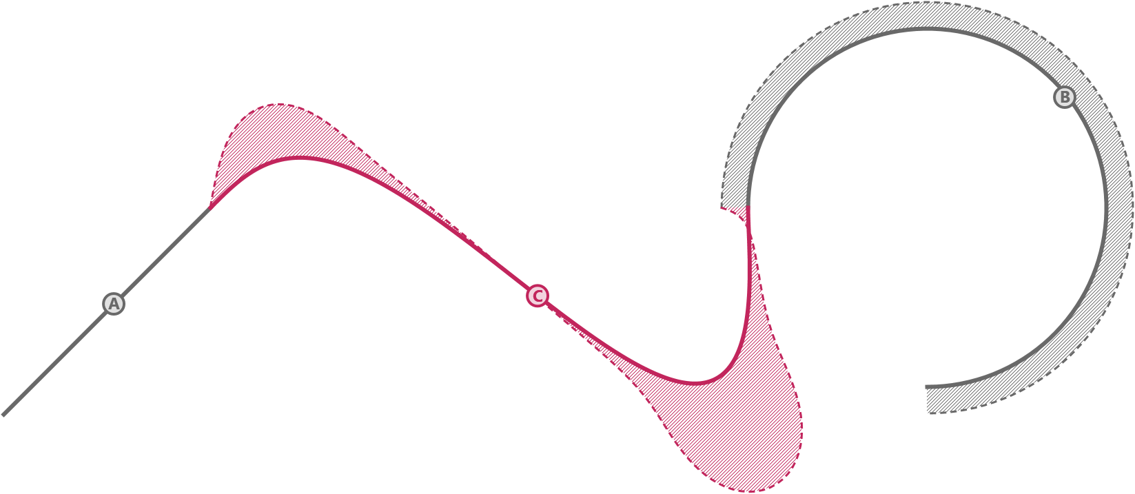
A single line cannot possibly satisfy four constraints at once as it has no degrees of freedom left after creating a $G_{0}$ connection. Hence, a different type of curve is needed for a $G_{1}$ connection. Multiple types of curve could work, for example degree-3 Bezier splines (not shown here), or bi-arcs, as per Figure 3.

A bi-arc consists of two circular arc segments, which at their point of contact are tangency continuous. The tangent directions at the end points of the bi-arc can be adjusted by varying the radii of the two component arcs. Thus a bi-arc has a higher degree of freedom than a line segment and can be used to satisfy all four constraints required for $G_{1}$ continuity.

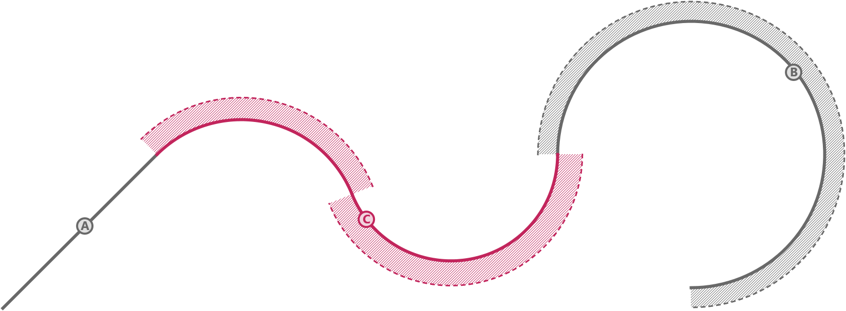
Figure 3. A tangent-continuous bi-arc connecting segment with curvature graphs.

It is impossible to cut oneself on a $G_{1}$ blend and circles tend to be easy and cheap to manufacture, but it is still a highly visible transition. There will be a notable difference in the shading and lighting on either side of a $G_{1}$ break, and especially reflections will be very jarring. Any object made out of reflective material will in fact appear to possess only positional continuity, due to the sharp break in the mirrored imagery.

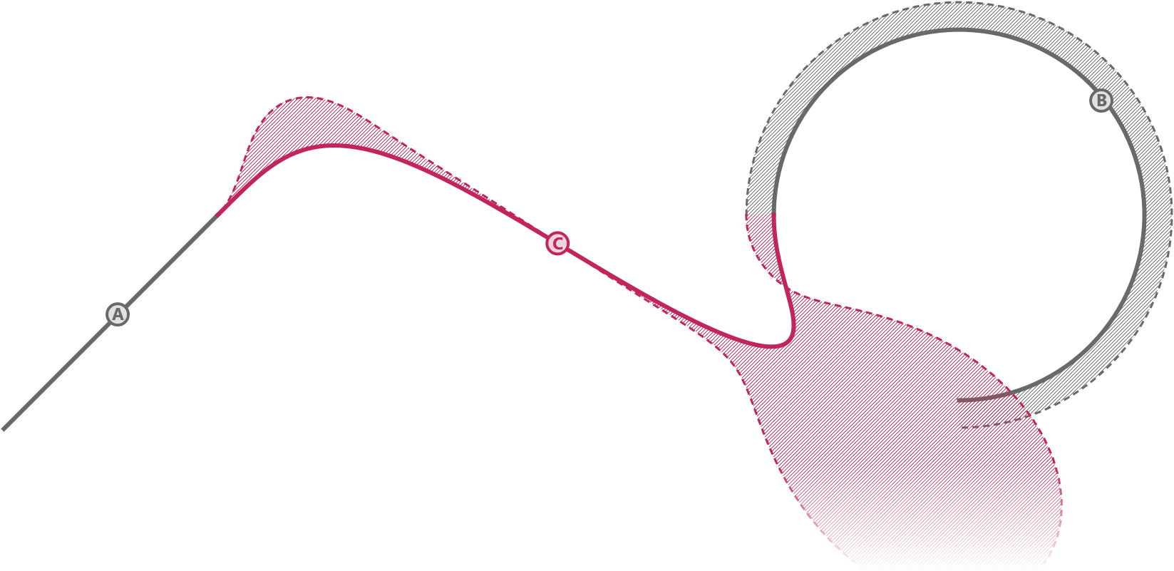
For a reflective object to appear smooth from a stationary vantage point, at least $G_{2}$ , or curvature continuity is required. In almost all cases this means that the connecting segment must have smoothly varying curvature along its length. Bi-arcs cannot provide this as they are made up of circular arcs, and circles have constant curvature everywhere. Degree 5 NURBS curves, on the other hand, can smoothly interpolate between position, tangency and curvature all at once, which of course adds two extra constraints:

The start of C must be coincident with the end of A.
The end of C must be coincident with the start of B.
The start of C must be parallel with the end of A.
The end of C must be parallel with the start of B.
The start of C must have the same curvature as the end of A.
The end of C must have the same curvature as the start of B.

This can be seen in Figure 4, where the curve itself has positional and tangency continuity, while the curvature graph no longer exhibits the sudden jumps at the segment transitions. The connecting segment starts out with zero curvature since it connects to a straight line without curvature, then varies the curvature drastically along its length, even flipping the sign twice creating inflection points, but ends up with the exact same curvature as the B arc where they meet.

Figure 4. A curvature-continuous curve with curvature graphs.

The curve itself may now seem perfectly smooth to the naked eye, but it is hard to miss the kinks in the curvature graph. At the transition from A to C and from C to B, the graph exhibits positional continuity only. That is to say, at the transition points the curvature of the segments on either side is the same, however the rate of change of the curvature is not. In the real world this would manifest as a choppy movement of reflections visible on the shape. This is why automotive design, which deals with reflective objects often seen in motion, relies on higher degrees of continuity than $G_{2}$ to make their products appear completely smooth.

A NURBS curve of degree 7 can provide a connection which smooths out even the curvature’s rate of change, as per Figure 5. For most applications this is sufficient. However in addition to this $G_{3}$ blending, Rhino provides one higher level of continuity based on degree 9 NURBS geometry, which ensures that the rate of change of a reflected imagery's acceleration across a surface is smooth. These higher degrees are called jerk and yank respectively in the Rhino code, but these terms are not used in the interface. Nor is this a particularly accepted standard terminology in the world at large.

Figure 5. A jerk-continuous curve is characterised by a lack of kinks in the curvature graph of the curve.

The concept of curve continuity can be transferred from two to three dimensions without significant changes. The only additional complication with curves in three dimensions is that at a given transition the numeric curvature of two adjacent curves may be equal, but the direction of curvature before and after the point may be different. It is not enough to merely compare the curvature magnitude, the curvature orientation must also be taken into account.

Surface Continuity

The concept of continuity does get quite a bit more hairy when applied to surfaces in three dimensions. Evaluating continuity at some point on the interior of a single surface is already quite a complex matter, as the continuity level may depend on the choice of trajectory through the point of interest. There is only one way to walk along a curve, but surfaces allow for an infinite amount of different paths.

If that was not bad enough, surface continuity becomes especially tricky when trying to measure continuity between adjacent surfaces. When curves are joined together end-to-end the result can be treated as a single, longer curve. However, when surfaces are joined at their edges the result is a poly-surface, whose individual patches may not align at all, as shown in Figure 6. I.e. the (u,v) directions of one surface may be flipped or opposite to those of its neighbour, or even at some arbitrary angle. This means that even if we find a natural or meaningful way to approach the point of interest from one surface, as soon as we cross over into the other surface’s interior the trajectory we were on is no longer a sensible one.

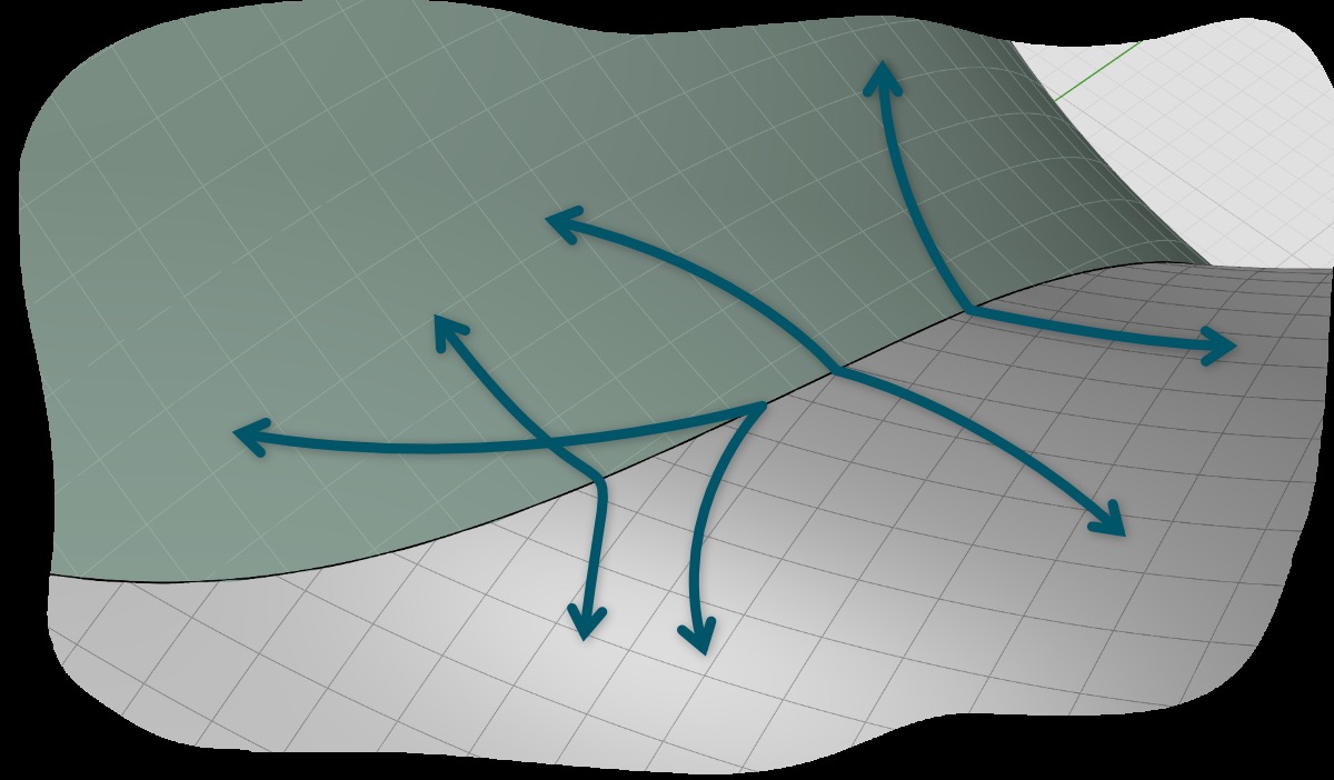
Figure 6. Continuity at a point on the boundary between faces must take into account the (uv) orientations on either side.

Comparing tangencies and curvatures on either side of such a complicated edge is quite an involved procedure, and beyond the scope of this topic.

Analytic Continuity

Analytic continuity is the foundation on which geometric continuity is built. The two concepts are practically the same, but the analytic approach enables a more rigorously mathematical definition of continuity, which is important when developing algorithms for measuring or adjusting continuity. Instead of tangible geometric ideas like shapes and kinks and reflections, which are easily understood but difficult to encode, analytic continuity relies on functions and derivatives and integrals which are harder to grasp but easier to write down. Incidentally, "analytic" in this case is a reference to the mathematical field of analysis.

Analytically speaking, when two functions intersect, i.e. they yield the same y value for a specific x value, the continuity at the point of intersection is a direct consequence of the number of derivatives of those two functions which also intersect at that same x value.

Consider the two cubic polynomials f(x) and g(x) drawn in Figure 7. They intersect at three points and it is fairly obvious visually that all three intersections happen at an angle, meaning the tangents of f(x) and g(x) are different from each other at all three locations. Since we are now speaking the language of analysis, we should say that the derivatives fʹ(x) and gʹ(x) do not intersect at either of the three locations where f(x) and g(x) intersect.

The derivatives do intersect at $x = 0$ and $x = 2$ , which means that at those x-coordinates the two cubics are parallel. However for those derivative intersections to matter for continuity, they must occur at the same x parameters as the function intersections.

As the number of intersecting derivatives at $x = 1$ is equal zero, the continuity of these two functions at $x = 1$ is $G_{0}$ . That is, if we were to construct a single curve defined by f(x) for all values to the left of $x = 1$ and g(x) for all values to the right, that compound curve would have a kink at $x = 1$ .

Figure 7. Two cubic polynomials with three intersections, all of them positional.

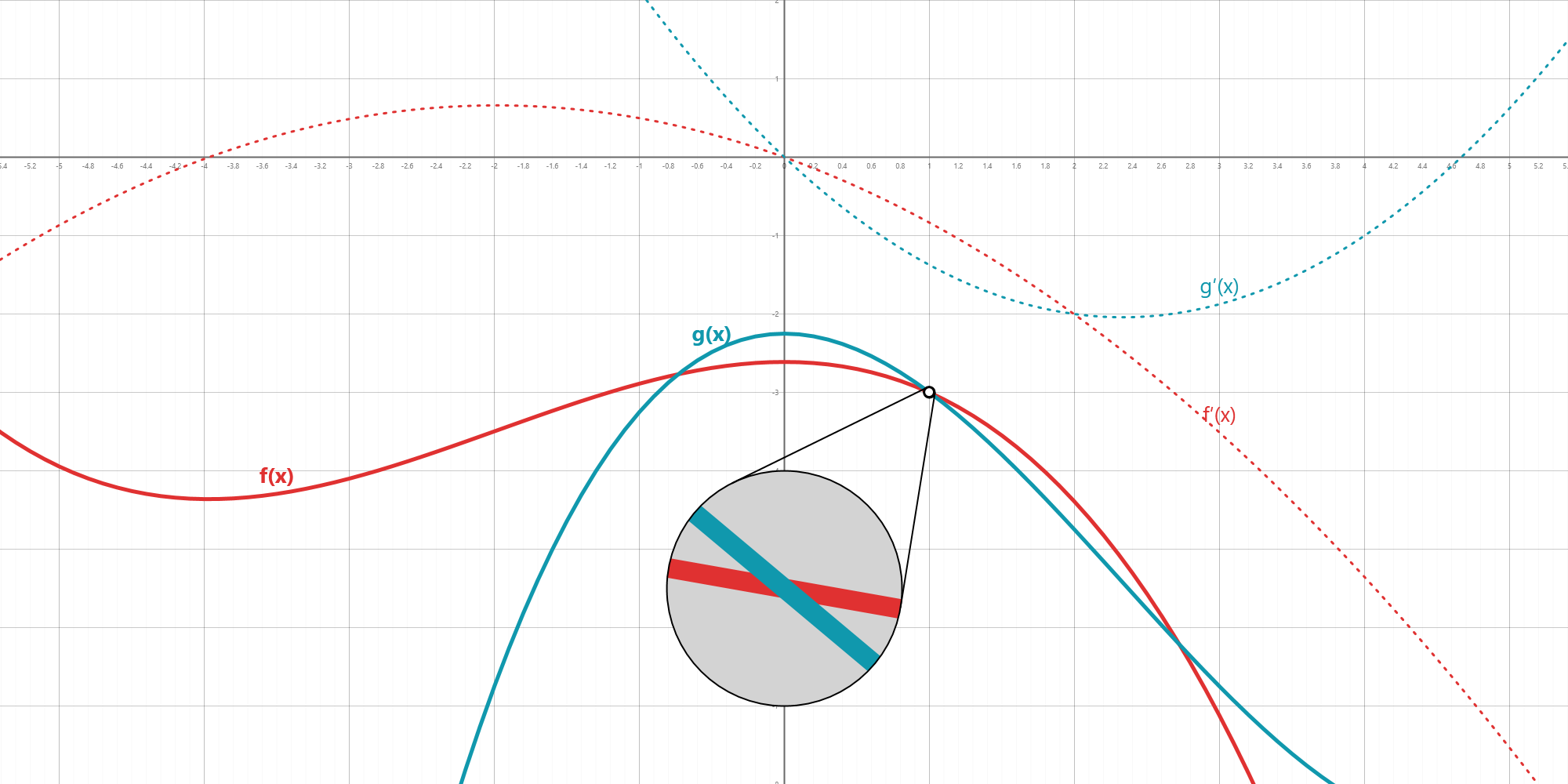
If we adjust the blue cubic somewhat, we get Figure 8. There are now only two intersection points left between f and g, and the intersection at $x = 1$ has become a glancing hit; the blue curve is above the red curve both before and after the intersection. In other words, the positions as well as the tangents of both functions must be equal at this point.

This can be verified by looking at the derivatives, which now also exhibit an intersection at $x = 1$ . Yet, the intersection of the derivatives fʹ(x) and gʹ(x) at $x = 1$ happens at an angle, meaning the second order derivatives (fʺ(x) and gʺ(x), not drawn) cannot be equal at $x = 1$ . Thus this intersection must be classified as $G_{1}$ or tangency continuous. The subscript number merely represents the amount of intersecting derivatives, there is nothing more to it.

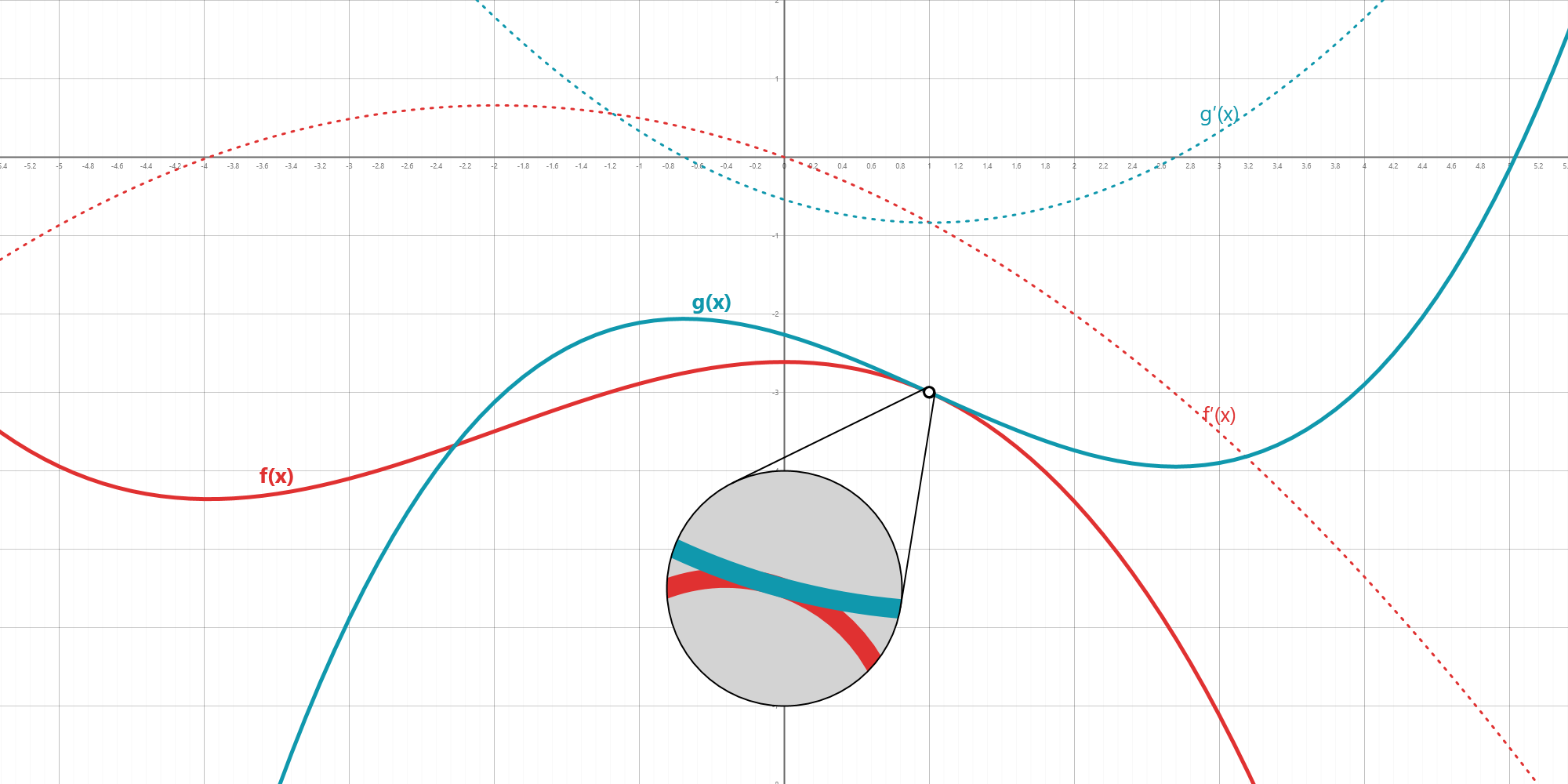
Figure 8. Two cubic polynomials with a tangent-continuous intersection at <math><mrow><mi>x</mi><mo>=</mo><mn>1</mn></mrow></math>, evidenced by the fact that the dotted derivatives also intersect at <math><mrow><mi>x</mi><mo>=</mo><mn>1</mn></mrow></math>.

Performing the same trick one more time yields cubics whose first and second derivative pairs all converge at $x = 1$ , yielding a $G_{2}$ continuity. As can be seen in Figure 9, the parabolas associated with the first derivatives are now glancing at the point of intersection.

Also note that once again we have lost an intersection between the main curves. The two cubics f(x) and g(x) now only meet at a single x parameter. This heavily implies that there is a trade-off between continuity and flexibility. If we wish to increase the continuity, we lose a certain amount of control over the exact shape of the curves. This is why it is not possible to obtain a $G_{3}$ level intersection between two cubic polynomials, as the increased continuity from $G_{2}$ to $G_{3}$ would mean the loss of the one remaining point of intersection. Both equations would have to be completely identical for their third order derivatives to also intersect, meaning the whole notion of continuity at a single intersection point is out the window.

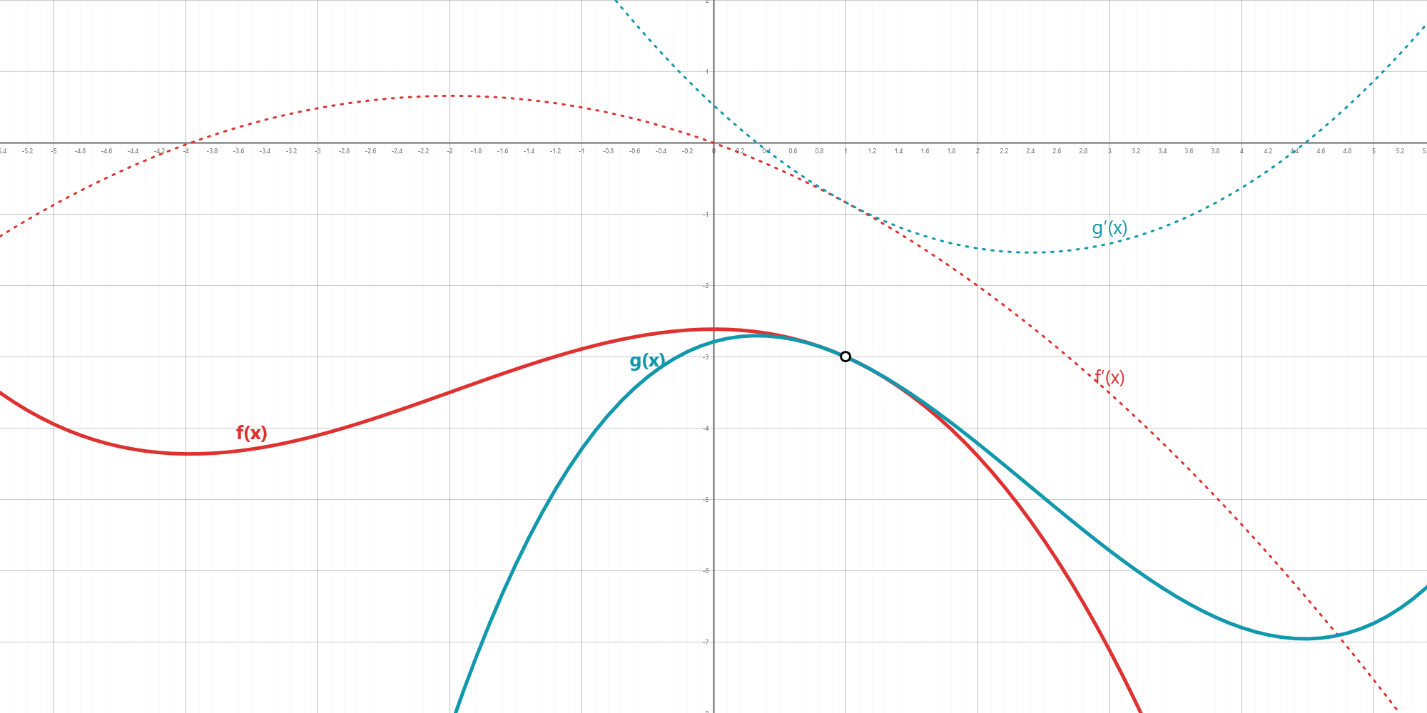
Figure 9. Two cubic polynomials with a curvature-continuous intersection at <math><mrow><mi>x</mi><mo>=</mo><mn>1</mn></mrow></math>, evidenced by the fact that the dotted derivatives exhibit a glancing intersection at <math><mrow><mi>x</mi><mo>=</mo><mn>1</mn></mrow></math>.

Since NURBS curves and surfaces are fundamentally constructed from polynomial equations just like the ones used in this section, it now becomes obvious why smoother blends require higher and higher degrees of NURBS geometry. It is literally impossible to create a $G_{2}$ continuity using only degree=3 curves as there aren’t enough derivatives to tweak. If curves or surfaces must exhibit Gₙ smoothness, at least one of them must have degree n+1 or higher.

Conclusion

To achieve high levels of continuity in shapes, one must rely on more complex curves and surfaces, that is, curves and surfaces with high NURBS degrees. One also loses a great deal of control over the form, as each additional level of continuity places more and more constraints on the local shape. It is therefore important to know what the minimum or acceptable level of continuity is for a particular design, and how to guarantee that level and no more.