Most geometry in Grasshopper is constructed explicitly; a radius must be chosen before a circle can be made, end points must be determined before a line is made, angles are computed before a rotation is applied, and so on. Every step computes its result from the steps leading up to it. A constraint system reverses this approach; initial shapes are drawn only very roughly and inaccurately, then constraints are declared which cause the shapes to be moved and scaled and rotated until the constraint demands are met.
These constraints typically specify simple relations between two entities in a single drawing. For example a constraint may require that two lines have the same length, or that two arcs share the same centre point, or that a line and a circle must meet at a tangent point. Once constraints are added, a constraint solver will attempt to tweak the initial shapes until all demands are satisfied simultaneously.
This topic explains what constraint systems are, what the solver in Grasshopper 2 can and cannot do, and how a constraint system is built with the Constraint System component. Details are covered in separate topics:
- Degrees of Freedom explains how much a constraint system is still allowed to move, and what happens when rules conflict with one another.
- Constraint Geometry describes the shapes that make up the geometric part of a constraint system.
- Constraint Rules describes the various constraints that make up the rule-based part of a constraint system.
- Constraint Inputs explains how dimensions and fixed points are driven by component inputs.
- Constraint Outputs explains how curves, points and measurements are sent to component outputs.
No prior knowledge of constraint solving is needed, but the reader is expected to be familiar with basic planar geometry such as lines, circles and arcs.
What is a Constraint Solver?
The core notion is that every shape can be described by a handful of numbers, and those numbers can be related to each other using arithmetical equations. A line segment is defined by four numbers; the and coordinates of both its end points. Meanwhile a circle requires only three numbers; two for the location of the centre and one for its radius.
A constraint affecting a shape is an equation involving some of those numbers. For example, a line from to is horizontal when . A constraint solver takes all the numbers and all the equations in a system, and finds the values for those numbers that make every equation true at the same time.
There is usually more than one valid answer. A line with a horizontal constraint and a length constraint of units can be placed anywhere in the plane without violating either of those constraints, so the solver picks the solution closest to the initial configuration. This is why constraint systems feel fairly natural to edit. Figure 1 shows that when the corner of a rectangle is dragged, the rest of the rectangle moves just enough to retain the rectangularity, and not a milliunit more. Humans develop an intuitive feel for changes that minimise action just by interacting with physical, real world objects.
Constraints make drawing certain shapes significantly easier than the regular Grasshopper approach, especially when tangencies or angles or interrelated dimensions are involved.
Constraints vs. Goals
Users of Kangaroo will recognise the idea of goals pulling geometry into different shapes. The two approaches look superficially similar but work very differently under the hood. Kangaroo simulates a set of forces, where each pushes and pulls on the points in the system. Those forces are first averaged per point and then applied all at once. This process is repeated until the system as a whole converges on a stable state. Goals in Kangaroo have strengths, and when they disagree the result is a balancing act between opposing forces.
The constraint solver does not simulate anything. It treats all constraints together as one system of equations and solves that system with arithmetic operations, typically arriving at the answer in only a handful of steps. Constraints do not have strengths: they either hold or they do not. When they cannot all hold, the solver still attempts to find the nearest compromise, but it reports how far off that compromise is and which constraints conflict. However, that compromised configuration is unlikely to be a useful one. Unlike Kangaroo, a constraint solver is not really suitable for dealing with conflicting demands.
See the Degrees of Freedom topic for a more in-depth explanation of under- and over-constrained systems.
Solver Envelope
The constraint solver which ships with Grasshopper 2 is a new constraint engine and has a fairly limited set of features, almost all of which will be familiar to anyone who has used constraint CAD editors before. The engine can:
- Solve planar drawings made of points, lines, circles, arcs, bends and guides.
- Enforce dimensions such as distances, lengths, widths, heights, radii, and angles.
- Enforce relations such as horizontality, perpendicularity, tangency, concentricity, and so on.
- Keep a drawing valid while parts of it are dragged by the user.
- Have its dimensions and fixed points driven by component inputs. This bridges the gap between Grasshopper's parametric approach and the constraint system's rule-based one.
- Output curves, points and measured values from a solved system back into Grasshopper's parametric workflow.
- Report how much freedom a drawing still has, and find which constraints are redundant or conflicting.
Notable features the solver does not have include:
- 3D constraints. Only 2D drawings in user-specified planes are supported.
- Free-form curves. There are no NURBS curves, splines, polylines or ellipses, only straight lines and circular curves.
- Inequalities. Every constraint is always active; there is no way to state that a length must be at least units or an angle may not exceed .
- Plurality. Two circles can touch on the inside or on the outside, and a bend can bulge to either side. The solver always looks for the solution nearest to the current configuration and doesn't allow switching to or exploring different configurations.
- Regions. The outputs are curves, joined into chains and loops where they connect.
Degrees of Freedom
Every additional piece of geometry introduces some freedom of movement into a system, and every additional constraint takes some of that freedom away.
A single point can move freely in both the and directions, so it has two degrees of freedom, while a point which can only move in one direction only has a single degree of freedom. A fully unconstrained line meanwhile has four degrees of freedom, since both end points are free to move independently. However, once a line has been given a horizontal constraint, one degree of freedom disappears as the coordinates of the end points are no longer allowed to move independently.
The constraint editor keeps a running count of the remaining degrees of freedom. A drawing with no freedom left is fully constrained: it can no longer be changed except by modifying the constraints themselves. A drawing with some freedom left is classified as under-constrained, and can still be dragged into other configurations without violating any of the constraints. Meanwhile, over-constrained drawings have so many constraints that some of them are no longer able to reduce the freedom of the system. That can be harmless when the extra constraints are redundant, but when they conflict the drawing typically cannot be solved at all without large remaining errors.
Constraints which do not remove any freedom because they duplicate already existing constraints are redundant, and usually highlighted by the editor as such. Though note that a redundancy always involves at least two constraints, while only one of them is highlighted. All of this is explained in more detail in the Degrees of Freedom topic.
Building a Constraint System
A constraint system is built in five steps. Though the order is pretty flexible, and in practice drawing, constraining and naming are mixed freely.
- Place a Constraint System component on the canvas, and double-click it to open the constraint editor.
- Draw the geometry roughly, using the shape tools. Shapes only need to look approximately right; the constraints will tidy them up.
- Add constraints until the shapes behave as intended. Drag things around to find out which parts are still free.
- Assign names to the dimensions and fixed points that ought to be controlled from Grasshopper values. Every name becomes an input on the component.
- Switch to
Output modeand give codes to the curves, points and measures that should be outputted from the Constraint System component. By default all standard curves are outputted, which may be sufficient.
The Constraint System Component
The constraint solver in Grasshopper 2 is not usable via components that create shapes and constraints. This is a marked difference from how Kangaroo is used, which sits entirely within the parametric environment Grasshopper provides. Instead, a constraint drawing must be made by hand using the Constraint System component.
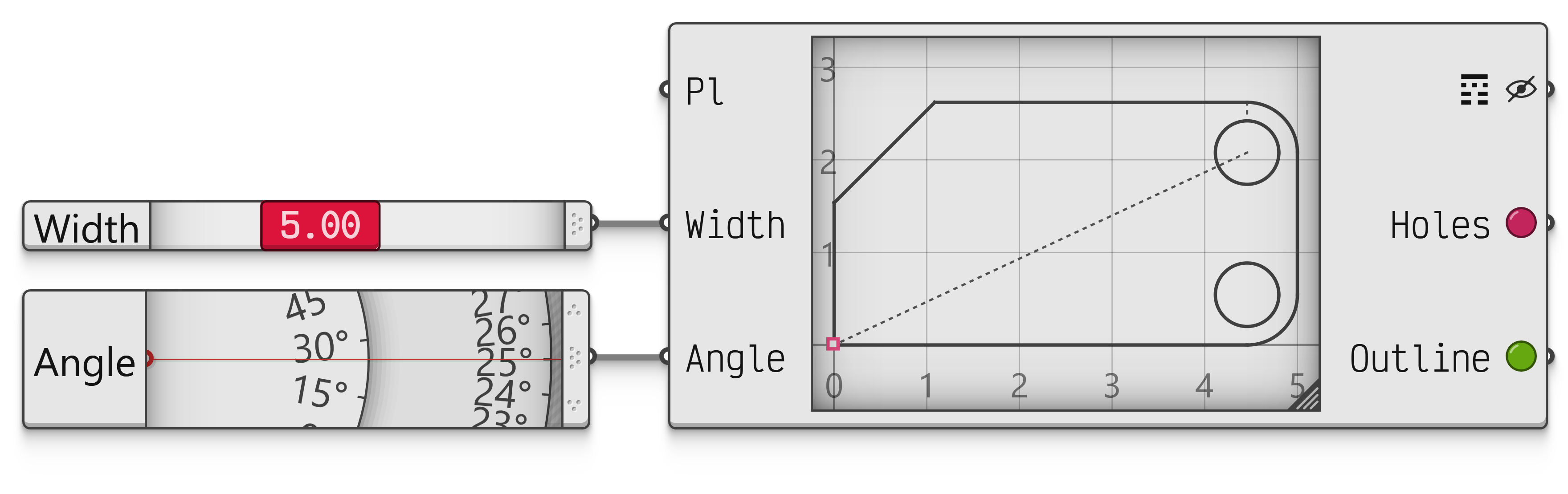 Interactive in Grasshopper 2
The constraint editor window visible in figure 5 is opened by double-clicking the drawing on the component, and it provides access to all the drawing and tagging and measuring tools needed to embed a constraint system into a Grasshopper file.
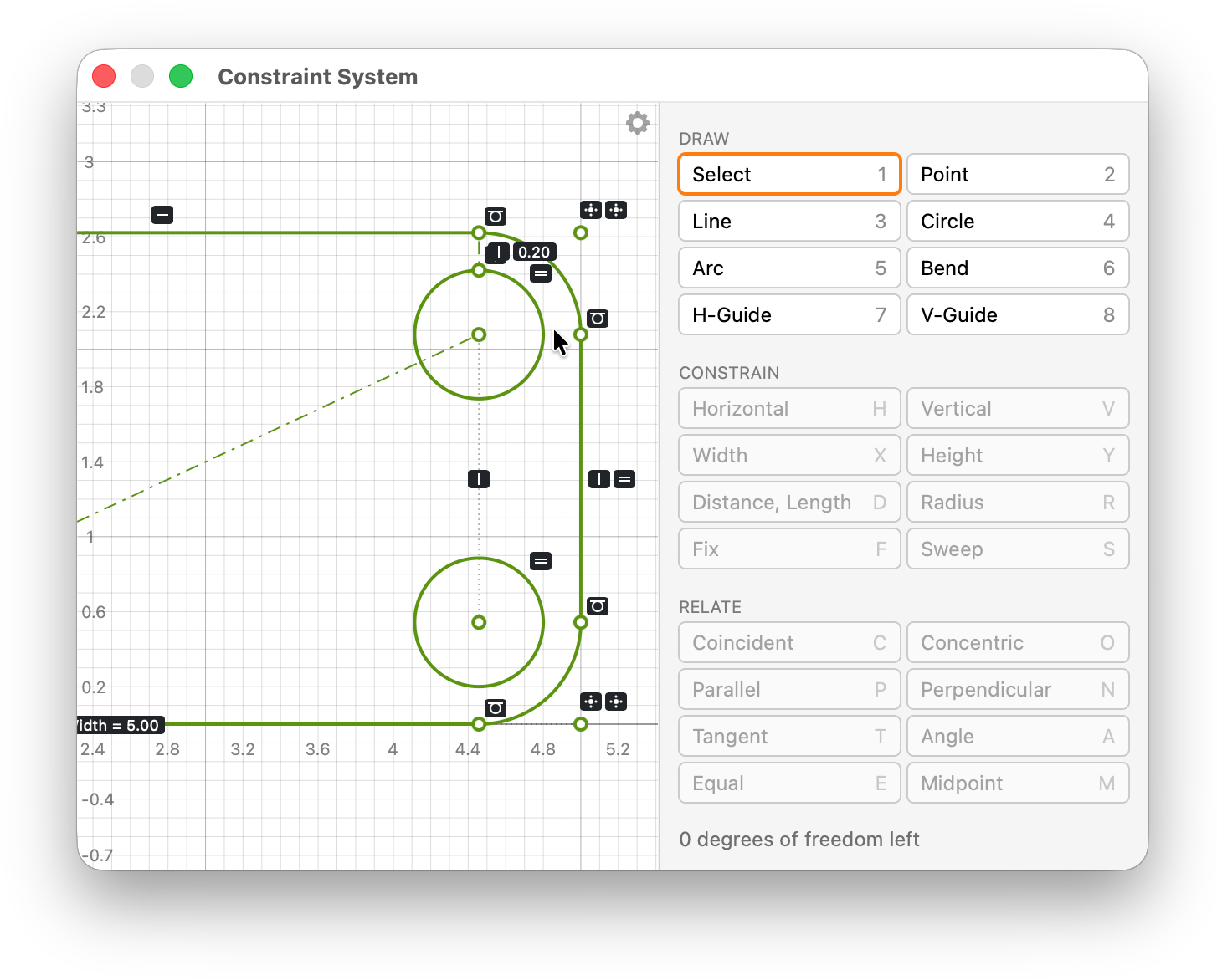
The component always has a Plane input, which places the drawing in 3D space, and an Edges output, which contains all regular curves of the drawing joined into chains and loops. Custom inputs and outputs are added and removed automatically as names and codes are added to or removed from the drawing.
Constraint drawings can be loaded and saved from the component popup menu as plain text files.
When a constraint system cannot be solved for the current input values, the component reports an error. When it can only be solved approximately, within the allowed error, the component reports how far the results are off. See Degrees of Freedom for an explanation of the allowed error.