A colour model is a collection of rules and ideas used to describe individual colours and the relationships between them. This is intentionally vague since colour models come in so many different flavours. When a colour model becomes precise and unambiguous, it will be referred to as a colour space, although sadly the distinction is not always entirely clear. This topic will discuss several models including some of their emergent spaces, as well as some of the core concepts of colour representation.

A mere collection of named colours without equations or interrelationships is a colour system or colour palette rather than a colour space. Here, too, the distinction is not necessarily unambiguous, but generally speaking if an entity awards names rather than numbers to colours it is probably a system. Examples of colour systems are RAL, Adobe Pantone, OpenColor, and X11.

Models —and especially spaces associated with them— can be either discrete or continuous, they can have gamut limitations, and may define a variety of relationships between colours such as distance, similarity, or comparisons between saturations or brightnesses.

A discrete colour space only allows for a finite amount of unique colours. On finite computers every space is necessarily discrete, but usually spaces with integer variables are treated as discrete, while spaces with floating point variables are treated as continuous.

The gamut of a colour space represents the boundary beyond which colours can no longer be represented. For example a model might restrict itself to pure spectral colours only, in which case greys, browns, purples, and other blended colours fall outside its gamut.

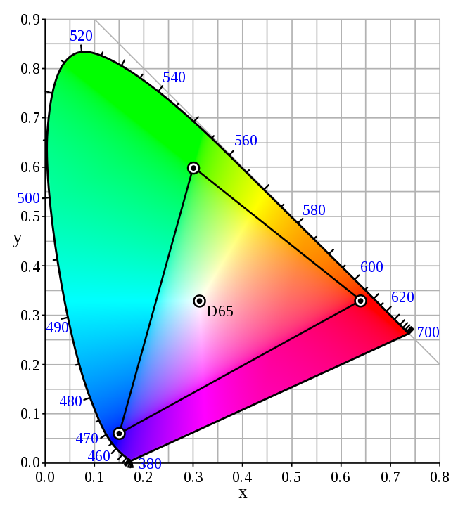
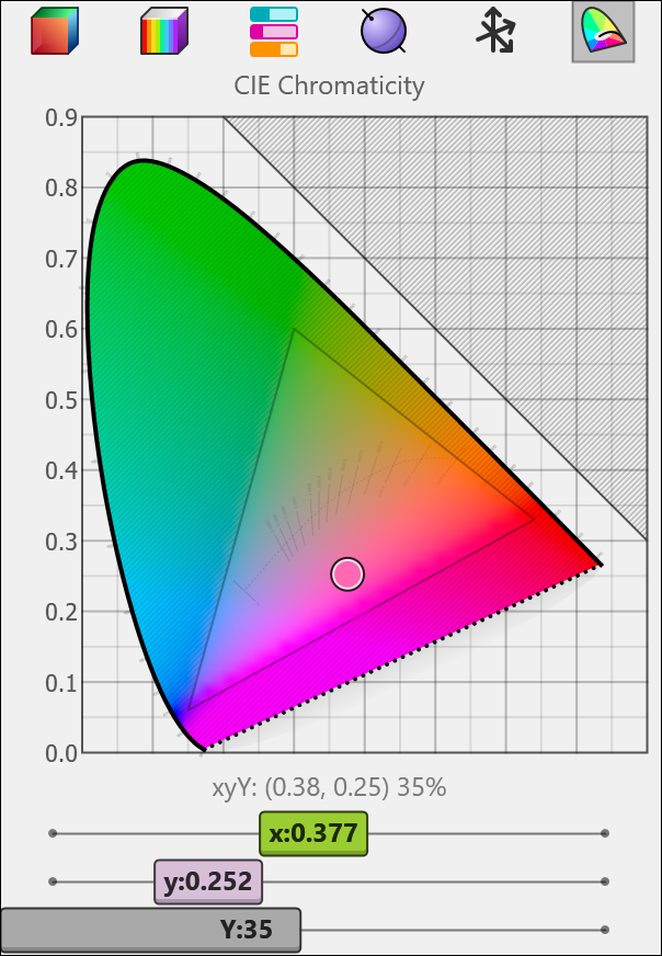
As Figure 3 shows, the gamut of the standard RGB colour space is but a small triangle within the space of all colours visible to standard humans. From this it follows that computer screens are pretty adept at showing purples, reds and oranges, but fall short in the greens and cyans.

Model Categories

Colour models broadly fall into three categories; physical, technological and biological. Physical models are concerned with the distribution of energy within a spectrum, usually represented by spectral curves. Such curves specify the amount of energy associated with each relevant portion of the electromagnetic spectrum. Although physical models are used in computing when simulating real world effects (for example in photorealistic rendering), they fall outside the scope of this document.

This leaves technological and biological models, both of which are surprisingly recent developments, no more than a century or so old. Technological models are associated with devices, such as printers or screens, whereas biological models are based on the characteristics of the (human) eye.

There have of course been many colour systems developed well before the 20th century, but these were primarily artistic or linguistic formulations, which did not allow for a formalised, mathematical approach. Most notable amongst these early attempts is the Munsell system, which exists somewhere on the boundary between systems and models. The Munsell system was sufficiently coherent and rigorous to serve as inspiration for several modern models.

CMYK Models

With the advent of standardised colour printing, technological models based on specific inks and dyes were developed. Today, most people who use computers semi-regularly will be familiar with the CMYK model, but may remain unaware that there are many hundreds if not thousands of spaces associated with the model, often limited in use to a specific machine, process, paper type, or company.

The CMYK model itself, however, is a widely used standard and describes colours by specifying the amount of cyan, magenta, yellow and key (black) ink or dye in a mixture or layering. As such the CMYK model belongs in the class of subtractive colour models which are based on the notion that specific materials called dyes absorb specific wavelengths of light, and that a mixture of various dyes will absorb all the wavelengths of its compounds. More dye means more light is absorbed, which yields a darker result on paper as there is less light bouncing off the material. Because of this, the model is subtractive; it simulates the removal (by absorption) of light.

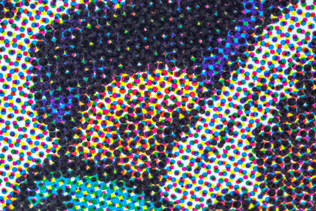
CMYK spaces are specific instances of the Subtractive Colour Model in that they must specify well-picked primary colours. Since different colour printers may choose to operate on different inks, each machine requires a specific, tailor-made CMYK space.

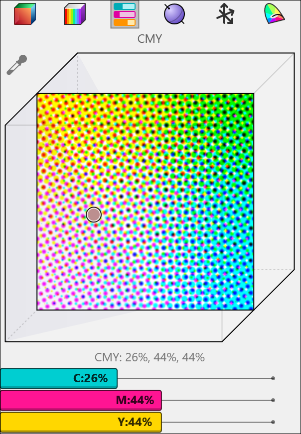
There is a lower-dimensional version of the CMYK model without the key axis, called CMY. In this model, black and grey colours are specified using equal amounts of cyan, magenta and yellow. CMY is mathematically identical to CMYK, but rarely used in actual printing as coloured inks are much more expensive than black ink. The CMY model is available in the grasshopper colour picker though, whereas the CMYK model is not.

Other technological colour models in common use today typically originate from display devices including analogue colour-TVs with cathode-ray tubes, or digital screens such as thin-film-transistor LCDs, plasma screens, and more recently OLED devices. Models and spaces associated with these devices are designed specifically to cover the available gamut, ensuring no bandwidth is wasted on colours which fall outside the capabilities of the device. But there is also a need for standardised models for when colour data must be shared or when it exists divorced from a specific device.

RGB Models

Chief amongst these standardised models is the RGB colour model. The RGB models describe colours by specifying the amount of red, green and blue light in an emission. More light equals brighter colours, which is why this model is additive rather than subtractive.

There are various competing RGB spaces advanced by companies like Microsoft, Kodak and Adobe, but unless one is involved in professional printing these distinctions are not relevant. It is, however, important to know the difference between linear-RGB and standard-RGB or just sRGB for short. The most straightforward formulation of an RGB model assumes a linear relationship between the numeric values along the red, green, and blue axes and the amount of light of that colour emitted. Yet such a relationship yields an inefficient colour space for a discrete, 8-bit-per-channel device, since large areas of this space are very dark.

Dark colours look more similar to the human eye than bright colours, so a different formulation of the RGB model was proposed to remedy this drawback. Adjusting the values in the RGB space in non-linear ways compresses the dark regions, thus yielding the sRGB space, which has a wider variety of bright colours. These adjustments are a form of gamma correction. The sRGB space isn’t mathematically tidy, but does a good job of providing a wide range of visually distinct colours within the 8-bit constraints.

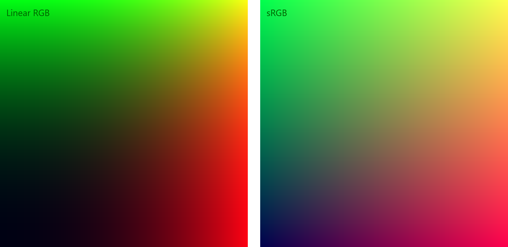
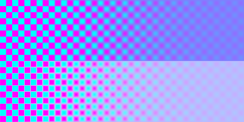
Apart from high-dynamic-range colours, it is likely that any RGB colour you've ever come across was specified in the sRGB space, whether or not the ‘s’ is specifically prefixed. While sRGB is well suited for display purposes it ought not be used in operations involving image processing such as interpolation or blurring, since the artificial non-linearity frustrates any straightforward colour algebra. Figure 7 shows how a simple blurring operation introduces dark blue regions between magenta and cyan when it occurs in sRGB, as opposed to linear-RGB.

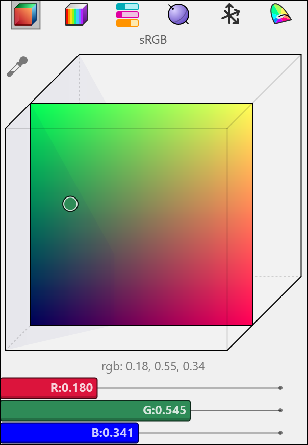
The grasshopper colour picker provides access only to the sRGB model, even though many behind the scenes colour computations occur in linear-RGB.

The XYZ Model

In the late 1920s various experiments were performed on human colour vision and the mixing of light, with largely similar conclusions. It is possible to simulate any pure colour —light of only a single wavelength— by combining the light from three monochromatic lamps; one blue, one green, and one crimson/red. Pure orange for example would be indistinguishable from a combination of 65% red, 35% green, and 0% blue.

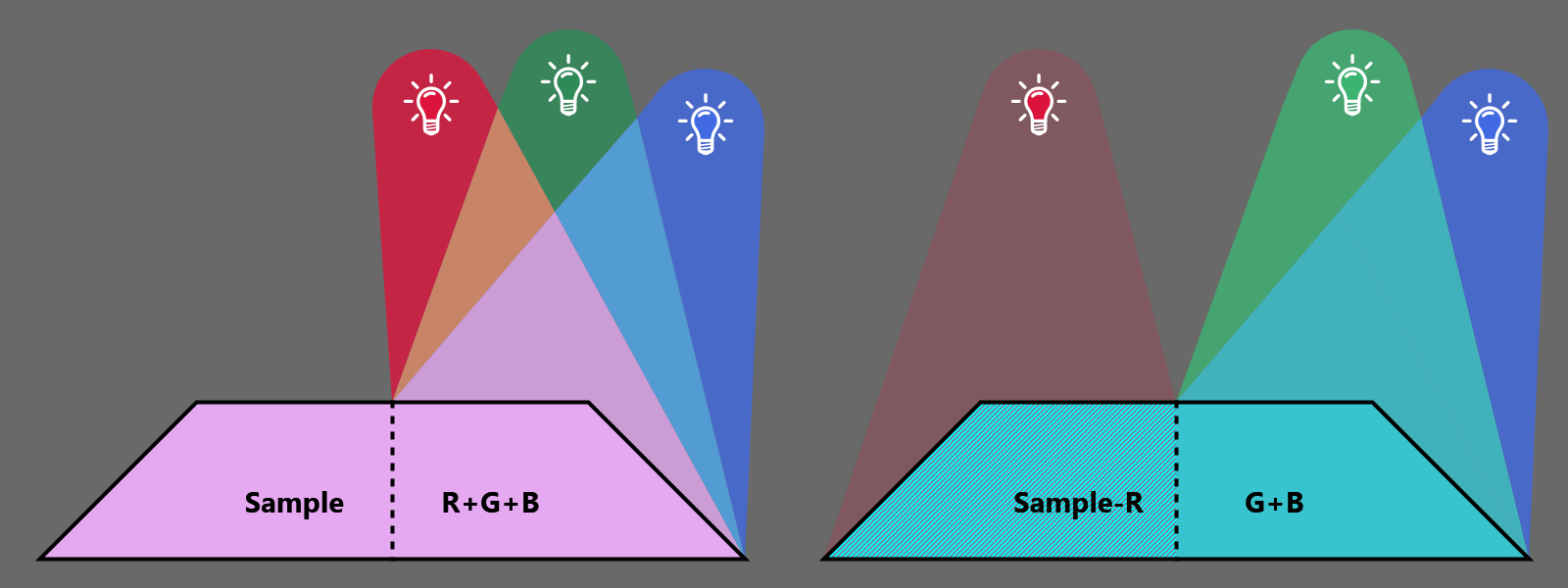
This is little more than the RGB model on a strong scientific footing, but these experiments yielded some inconvenient measurements standing in the way of neat mathematical equations which would cover the entire visible spectrum. For certain pure colours in the teal and cyan region of the spectrum, the amount of red light needed for a visual match was negative; anti-red. It may sound very esoteric but the explanation is rather mundane. There were no combinations of red, green and blue light that would yield a blend indistinguishable from cyan, but a match could be created using only blue and green, provided the red lamp was allowed to shine on the sample area, instead of the comparison area. Therefore the red must be treated as a negative value.

To overcome this problem of negative values in the equations of the colour space, the three axes associated with the primary colours in the RGB space had to be modified, yielding new primary axes called X, Y, and Z. They were given these awkward names because they are not real colours. The transformations required to conceal the negative values in the red component rotate the familiar RGB colour axes through a bizarre angle, leaving X, Y and Z as imaginary colours. Mathematically solid, physically impossible.

An understandable analogy for this mathematical sleight of hand might be the following; imagine you wish to specify all cities in Italy as a linear combination of three primary cities, say Rome, Genoa and Bolzano. Unless you allow for negative factors you are limited to the triangle with corners at R, G and B, and there are clearly many Italian cities outside of this triangle. But the point is that you cannot pick three cities within Italy whose connecting triangle would contain all other cities. You must pick your reference points outside of Italy. For example the triangle defined by Paris, Odessa, and Tripoli covers all Italian coordinates (all the real colours), but also many foreign ones (imaginary colours).

The upshot of this is that all colours visible to humans can be denoted as linear combinations of X, Y and Z, without any of the factors ever being negative. That is, the gamut of the XYZ space is larger than the gamut of all visible colours. Because of the mathematically solid formulation, the XYZ model often plays a pivotal role in the specifications of other colour spaces, or at least functions as a handy go-between when converting coordinates from one colour space to another.

By rotating the XYZ axes in yet a different way the Yxy colour model is created. Despite not being real, the XYZ primaries were at least in the vicinity of the familiar Red, Green and Blue primaries. In the case of Yxy the uppercase Y axis is oriented along the brightness direction of the colour space. That is, low values along Y yield dark colours and high values yield bright colours. The lowercase x and y axes get dragged along and in the process lose their distinctive characters, as they no longer describe a specific aspect of colour. The resulting colour space is available in the Grasshopper colour picker under the name CIE Chromaticity Diagram. This model is important since many legally or officially defined colour constraints (such as the colour of traffic lights or warning signs) are specified in Yxy coordinates. Do note that many colours within the Yxy gamut fall well outside the RGB gamut.

Luma-Chroma Models

With the advent of colour-TV, new colour models had to be developed to allow broadcasters to include colour information without making the program unwatchable on existing black-and-white-TV sets. This was achieved by separating the image brightness (or luma, or luminance) from the image colour (or chroma, or chrominance). This way the existing TVs would still only interpret and correctly display the black-and-white luma component of the signal, while new colour TV sets could overlay the chroma data. An additional benefit of splitting colours into luma and chroma components is that the human eye has great detail resolution for luminance contrast, but terrible resolution for chroma contrast due to the different density of rods and cones in the retina. Thus a broadcast signal can sacrifice chroma bandwidth in favour of luma bandwidth to produce an image whose quality appears much higher than it actually is.

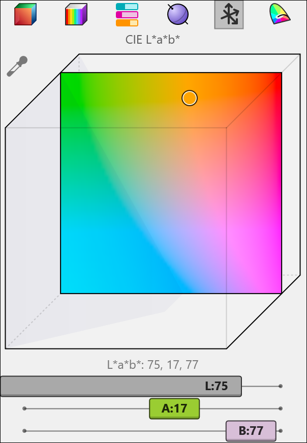
In Grasshopper, a common luma-chroma model called CIE L*a*b* (or just Lab for short) is available in the colour picker. The L stands for luma and ranges from zero (black) to one-hundred (white), although higher values could be interpreted as brighter-than-white colours. Meanwhile, the a* and b* axes together specify the chroma components. The a* axis represents a continuum between green and red, with negative values indicating green, positive values red and zero neither. This is a safe juxtaposition since a colour can never be both reddish and greenish; they are opposites. Meanwhile the b* axis performs a similar duty between blue and yellow.

Hue-based Models

Hue-based colour models seem to be a compromise between the technology based RGB model and the mental colour models humans construct within the privacy of their own minds. The conversion rules to and from sRGB are intentionally kept simple which goes some way towards explaining the abundance of these models in software. They appear more natural than sRGB, but not so natural as to require difficult mathematics.

The HSB/V, HSL and HSI models are all based on the principle of separating out the hue, saturation, and some kind of luma metric. The hue specifies to which ‘pure’ category a colour belongs. For example rose, vermilion, crimson and maroon are all related to pure red, and as such all have very similar hue values. Instead of a spectrum wavelength though, the hue is represented as an angle in degrees, with 0° being red, 120° green, 240° blue, 300° purple and 360° cycling back to red.

The saturation component tells us whether the colour is closer to the pure extreme or closer to grey. Finally the third component describes the brightness (or lightness, value, or intensity) of the colour.

At first sight this appears to be a sensible approach to defining colours, but by sitting on a fence halfway in between technological and biological, these models all end up having certain drawbacks.

First of all the cyclical approach to the hues is not physically warranted. The hue disc pretends to be a spectrum which has been bent into a circle, but the real spectrum starts with (ultra)violet and ends with (infra)red. To bridge the gap these models inject various shades of purple, which are not spectral colours at all; there is no purple in the rainbow. This in itself may not be that big of a problem, but it is emblematic of the middle-of-the-road approach. An additional problem with defining a cyclical progression of colours using an angle value is that colours with wildly different hue values may in fact be very similar, as 1° and 359° are in fact spatially close together, despite being numerically far apart.

A much more serious issue is that the hue value becomes meaningless when the saturation goes to zero. A completely desaturated colour is neither red, nor green, nor blue, nor purple, and yet it must have some hue value if it is to exist within these colour spaces. Unless great care is taken, and unless additional data is stored, a colour cannot be safely desaturated, then resaturated without reverting to some default hue.

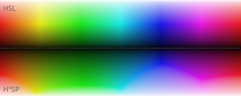
A further issue with the hue parametrisation shared by all these models is that it overwhelmingly emphasizes certain colour categories to the detriment of others. Green stretches for 60° before it becomes distinctly non-green, yet yellow and cyan must squeeze themselves into slivers no more than 10° wide.

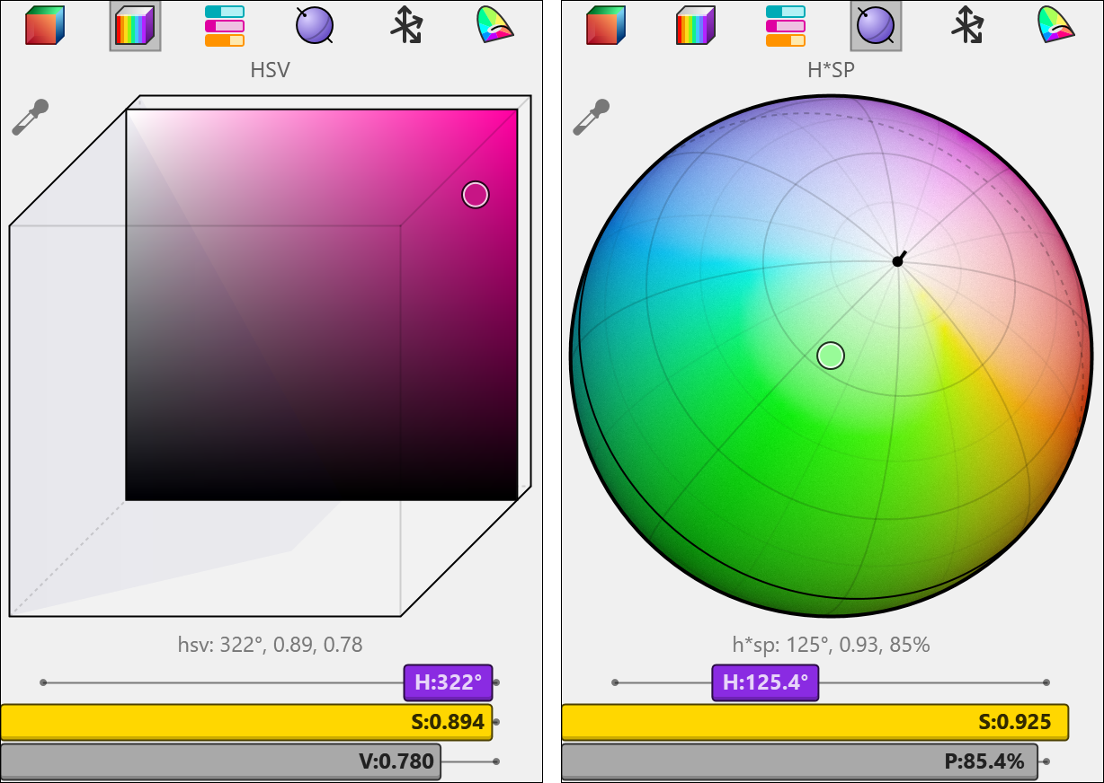
Despite these drawbacks, the Grasshopper colour picker does provide the HSV model since it is a very common one. In addition, a newly defined hue-based model called H*SP is provided as well, which relies on an adjusted hue-angle curve and a much better luma metric. The P stands for perceived luma and uses the luminance equations of the gamma-adjusted YCbCr colour space.

Conclusion

Colour is a complicated topic which sits at the intersections between Physics, Biology, and Technology. An in-depth understanding is happily not required to use the colour tools Grasshopper 2.0 provides, although a superficial familiarity with the concepts and terminology seems advisable. Grasshopper is not designed to be a graphics editing package and indeed lacks many of the fundamental features and algorithms a professional editor would expect, but version 2.0 does endeavour to treat the topic of digital colour with the respect it deserves and to open the door to continued development on this front.