This topic covers the syntax details for writing custom Display Rule instructions. For an introduction to the concept of display rules, see the Viewport Display topic.

General Syntax

Every set of display rules consists of an ordered list of instructions, each written on a separate line. Later instructions override earlier ones when there's a conflict, so if for example the instruction on line 3 assigns the colour Magenta to a specific shape, but the instruction on line 5 assigns Cyan to that same shape, the shape will appear cyan when displayed.

Individual lines may be empty, contain comments —indicated by a double slash at the start— or contain valid instructions. Below is an example of a completely valid rule set containing two comment lines, an empty line and three instructions.

1. // Display Rules for Material meta data validation
2. // Written by J. Salaryman on 2024/06/20
3.
4. Hide *
5. Show Material
6. Tint Material -> Lava

Display rule syntax always follows a specific template, except that some elements are disallowed depending on the specific command in question. Every instruction must start with a command followed by whitespace. Most commands then require a filter which restricts the instruction to specific shapes, followed ultimately by the arrow separator and a property:

command filter -> property

Some commands do not require or allow properties, while the Cite command is the only one which does not allow a filter. Using this template we can now interpret the instruction on line 6 in the example above. The command used here is called Tint, whose purpose is to override the display colour of shapes. The filter consists of the single word Material, which limits this command to only those shapes which have a material value in their meta data. Finally the property specifies that the colour Lava ought to be assigned to all shapes which pass the filter.

Commands

Table A lists all commands available for use in display rules. Note that Hide, Show, Tint and Wipe are compatible with all shape types, while Symbol and Size only apply to points, and Stroke and Dashes only apply to curves. The table also shows whether each command requires a filter or a property.

Command	Explanation	Filter	Prop
Cite	Import another rule set by name.	❎	✅
Hide	Hide shapes in the Rhinoceros viewports.	✅	❎
Show	Unhide shapes in the Rhinoceros viewports.	✅	❎
Wipe	Clear any display overrides assigned earlier.	✅	❎
Tint	Override the colour of unselected shapes.	✅	✅
Size	Override the size of point symbols.	✅	✅
Symbol	Override the symbols of points.	✅	✅
Stroke	Override the widths of curves.	✅	✅
Dashes	Override the dash patterns of curves.	✅	✅

Filters

Filter notation is the most complex part of display rule syntax, as its complexity can grow without bound. We might not be content to apply a rule merely to all shapes containing a Material value in their meta data. It is entirely likely that a much more specific filter with many individual checks is desired. For example, we might want to tint all wooden shapes on the north-facing façade of building B on floors 3, 4, 5 and 8. Filter notation must be flexible enough to encode such specificity.

But let us start simple. Sometimes an instruction is meant to apply to all the shapes that Grasshopper might draw in the Rhinoceros viewports. In this case a single asterisk is sufficient. Consider for example a display rule which tints all shapes which lack material meta data. This would be a handy visualisation in case we must check for missing meta data. This can be achieved in two steps; first colour everything red, then wipe the colour from all shapes containing the correct meta data:

1. Tint * -> Red
2. Wipe Material

The * in the first instruction ensures that all shapes are included, even those without any meta data. If instead we wanted to limit our instruction only to those shapes which have any meta data, additional single quotes will be required. When a single word —or a sequence of words— surrounded by single quotes appears in the filter, it is assumed to be the name of a meta data entry:

1. Tint '*' -> Red
2. Wipe Material

Any shape containing a meta data entry with a matching name will pass the filter, regardless of what type or value that entry has. We can employ comparison operators to make these filters more specific:

Operator	Meta data value test
= ==	Entry must match the given value
!=	Entry may not match the given value
<	Entry must be strictly smaller than the given value
<=	Entry must be smaller than or equal to the given value
>	Entry must be strictly larger than the given value
>=	Entry must be larger than or equal to the given value

Using comparison operators we can create a filter which hides all shapes without Floor meta data, or whose Floor number is less than two:

1. Hide *
2. Show Floor >= 2

It is possible to string multiple filters together with boolean operators, and to use round brackets to enforce a specific precedence. There are three boolean operators, and both C-style symbols and VB-style words are supported:

Word	Symbol	Explanation
And	&	Shapes must pass both filters
Or	|	Shapes only have to pass either filter
Xor	^	Shapes must pass exactly one filter

Using two partial filters and the and operator, we can amend the previous example rule to only show floors between two and six:

1. Hide *
2. Show Floor >= 2 and Floor <= 6

This chaining logic can be extended indefinitely. To return to the example used at the start of this section, in order to encode an instruction to "tint all wooden shapes on the north-facing façade of building B on floors 3, 4, 5 and 8", a rather complicated chain of partial filters is required. In the example below, the chain of partial filters is written on multiple lines to aid readability, but note that in order to be valid the entire instruction must appear on a single line:

Tint (Material = Wood)
      & (Building = B)
       & (Facade = North)
        & ((Floor >= 3 & Floor <= 5) | Floor = 8)
         -> Brown

Lastly, for those undeterred by complexity, filters may even consist of Grasshopper expressions. Any expression which evaluates to a boolean value can be put into a filter. For example, consider a document containing shapes with both Volume and Density meta data, we could construct a filter based on the weight of individual shapes. Assuming our units are all in order, multiplying the volume (in cm³) by the specific density (in kg/m³) and dividing by one million to convert from m³ to cm³ yields a weight in kilogrammes:

Tint Volume * (Density / 1e6) >= 250 -> Pink

Properties

Commands overriding the visual appearance of shapes require properties that specify this visual override. Properties are separated from the filter notation by the -> separator. Table B lists the types of properties that are allowed for the commands:

Command	Type	Property Notation
Tint	Colour	Names like Lava or Cyan are allowed, as well colour notation like rgb{200, 55, 0}.
Tint	Gradient	Names of gradients like Matter or Candy are allowed, as well as gradient notation like gradient{0=Red, 10=Black}. A from x to y instruction may be appended to change the domain of the gradient.
Size	Number	Any positive numeric value.
Size	Expression	Any expression yielding a numeric value. Names of meta data entries may be used as variables. For example 20 + Density or abs(Temperature).
Symbol	Text	One of the standard symbol names like cross, circle, plus, square and diamond.
Symbol	Integer	One of the integer values of the Rhino.Display.PointStyle enumeration as defined in the RhinoCommon api.
Stroke	Number	Any positive numeric value.
Stroke	Expression	Any expression yielding a numeric value. Names of meta data entries may be used as variables. For example max(Density, 3*Elevation).
Dashes	Text	One of the predefined dash pattern name: solid, short, medium, long and varying.
Dashes	Numbers	A list of numeric values representing the lengths of alternating dashes and gaps, for example 5,10,5,20.
Dashes	Expression	Any expression yielding a numeric value. Names of meta data entries may be used as variables. The result of the expression is used to measure both gaps and dashes. For example 0.01 * log(Decibels).
Cite	Text	The name of another rule set.

Some notes on expressions

Properties that accept expressions may face the issue that some meta data names violate acceptable variable notation. For example, names containing whitespace, punctuation, or names starting with numbers cannot be used as is in expressions:]

abs(Display.Stroke) + Material Density

In these cases, the offending names must be surrounded by single quotes in the expression to signal they are supposed to treated as individual external variables with custom names:

abs('Display.Stroke') + 'Material Density'

It is also possible to use x as a placeholder instead of the meta data name itself. So an expression like this:

min(50, 10 * log(Material Density + 1))

can circumvent notation issues and be made much more readable when x is substituted:

min(50, 10 * log(x + 1))

When the filter contains more than one meta data name, Grasshopper tries to always replace x with the first meta data name occurring in the filter. However, there is no guarantee of this succeeding, so in such complicated cases, it is probably safer to not rely on x-substitution.

Some notes on citing

The Cite command operates by invoking all the instructions in the named ruleset,. This process is recursive, so if the cited ruleset contains Cite instructions of its own, those will be invoked as well. It is therefore not allowed to create cyclical citations, since that would result in an infinite citation loop.

For a Cite command to successfully find a named ruleset, that ruleset must either exist within the same Grasshopper document, or it must be a standard ruleset which is saved on the user's machine. The Display Rules Editor allows users to turn any currently loaded ruleset into a standard one via the menu.

Do note that when standard rulesets are cited, the rules may stop working as intended when that file is shared with people who do not have those same standard rules.

Examples

This section will provide some functioning examples of display rules with varying degrees of complexity. You can drag the file previews from this window onto the Grasshopper canvas to load the files and tinker with the rules.

The first example file shown in Figure 1 explains how to associate numbers in meta data with a colour gradient. Each point in the collection is tagged with meta data containing a number which represents the distance from that point to the given circle. By using a gradient instead of a colour as the property for a Tint command, we can draw each point in a unique colour with a single instruction.

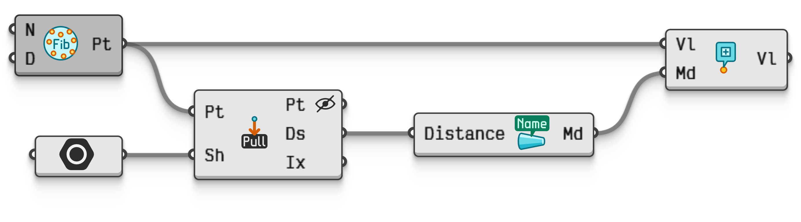Interactive in Grasshopper 2

To see this file in action, drag the above image into Grasshopper and open the Rule Editor via the Display->Display Rules->Rule Editor… menu.

The rule editor consists of three parts. The topmost control allows for active rules to be renamed, or for currently inactive rules to be made active. The middle control is a text field where the rules are typed, and the bottom-most panel shows a summary of all the meta data present in the current Grasshopper document, sorted by relevance. It is here we can see the distribution of meta data values, which is important information when creating rules.

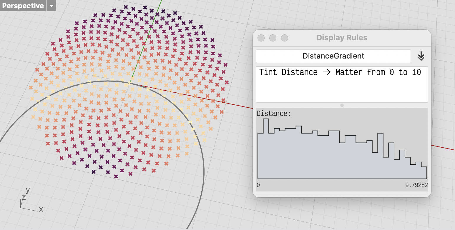
The bar graph in the meta data summary shown in Figure 2 shows that the Distance values vary from 0.0 to just under 10.0 units. Since this rule invokes the standard Matter gradient which has a domain from zero to one, it must resize the gradient lest almost all points are drawn in dark purple. By appending the from 0 to 10 resizing instruction, the domain of the gradient is amended to cover the entire distribution of distance values.

---

The second example shown in Figure 3 contains three rules, whose ordering is significant as their filters overlap. The file itself contains a collection of lines with meta data recording the distance from those lines to a point. The three rules all apply different dash patterns based on whether the line distance exceeds the given constant values 5, 7 and 10. The idea is to draw far away lines progressively fainter by using dash patterns with shorter dashes and longer gaps:

1. Dashes Offset > 5 -> 15 5
2. Dashes Offset > 7 -> 10 10
3. Dashes Offset > 10 -> 5 20

But note how all three filters are true if the Offset value is larger than ten. When multiple instructions are relevant to a single shape, the later ones override the earlier ones, which is why this rule set would not work if the instructions were reversed.

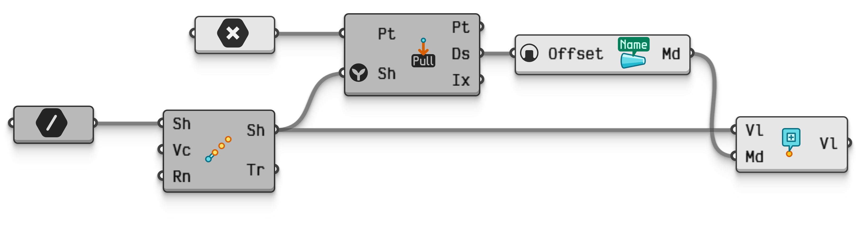Interactive in Grasshopper 2

---

This third example showcases the flexibility afforded by expressions in display rules. The file contains a grid of circles whose meta data values are sampled from a scalar noise field, with values fluctuating between zero and one. If we want to draw circles thicker where the noise is louder, we cannot use the meta values directly, as that would draw circles with at most a single pixel thickness, the thinnest possible width for drawing curves. Instead, the property will use an expression containing the variable x to amplify the curve widths up to fifteen pixels.

Stroke Custom -> x*15

Note that instead of x we could also have used Custom. The x variable is just a placeholder for the first meta data name to appear in the filter.

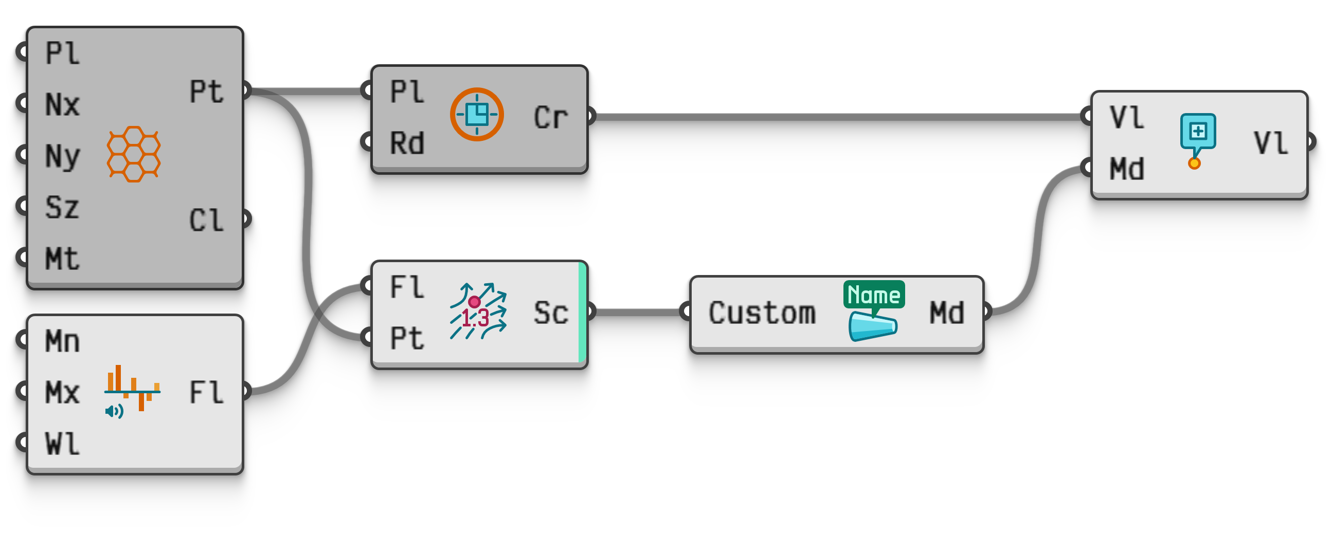Interactive in Grasshopper 2