In order to answer questions about geometrical objects and their interrelationships in space, such as "are two points coincident?" or "is this point to the left of that line?" coordinate systems need to be constructed. A coordinate is an ordered list of numbers identifying a location in space. A coordinate system is the set of equations required to convert a coordinate into a geometric point, and vice versa. The amount of numbers in a coordinate is often the same as the amount of dimensions of the associated space, but this is by no means a requirement.
Some of the earliest coordinate systems were invented by the Ancient Greeks. These were, however, shape bound systems and thus inextricably linked to specific individual shapes. One such example is using the major and minor axes of an ellipse as the basis for a coordinate system. The drawback with such an approach is that two or more shapes can not freely coexist in the same system. The orientation and sizes of any secondary shapes are subservient to the primary shape.
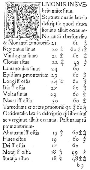
The notion of a coordinate system which pervades all of space and acts as a framework within which shapes can exist and move about is the invention of René Descartes. In 1637 he published a treatise on what is today called the Cartesian coordinate system. This was one of the most important events in the history of mathematics as it bridged the divide between two previously separate fields of study; geometry and algebra. When shapes can be described using coordinates, which are in turn described using numbers, it becomes possible to rephrase geometric problems in the language of algebra—and later calculus and analysis. And conversely it becomes possible to think about numerical problems geometrically.
The Cartesian system was the first of its kind, and remains the most commonly used coordinate system today. Many others have since been proposed, some meant for solving specific problems, some to fit a particular kind of space, and some merely for their mathematical beauty.
The Cartesian System
The Cartesian system has been the most common approach to the parametrisation of flat space since it was invented in the 17th century. An n-dimensional Cartesian system requires an origin point and n axis vectors—or just axes for short. All axes must be equally long and perpendicular to each other. The lengths of all axis vectors define the unit length of the coordinate system, in that all measured or computed distances are expressed in terms of multiples of this length. This is why all axes must be equally long, otherwise the measured size of a shape will vary with its orientation in space.
Despite the constraints placed upon the choice of axes, there are still different ways to set up a Cartesian system. Even in just two dimensions, once the first axis has been selected there still remain two possibilities for the second axis. It could be placed either 90 degrees clockwise from the first, or 90 degrees anti-clockwise. Both these choices fulfill the perpendicularity requirement. We can thus speak of clockwise and anti-clockwise (or counter-clockwise) systems in two dimensions.
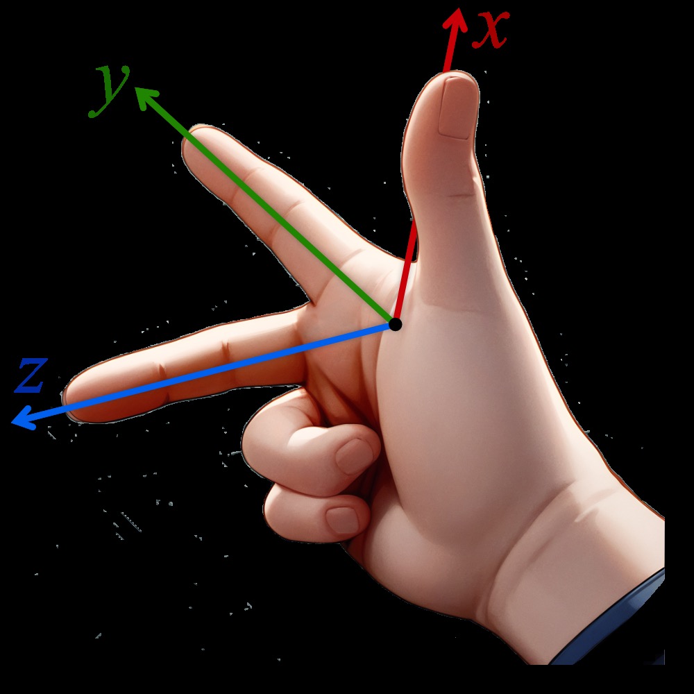
Similarly, in three dimensions there is also a choice of two opposite directions for the third axis. This leads to the distinction between right-handed and left-handed systems.
If the right thumb, index and middle fingers can be used to mimic the axis directions (thumb=X, index=Y, middle=Z), the system is right-handed. |
 |
These Cartesian rules are the reason why all planes in Rhinoceros and Grasshopper must have right-hand-oriented, perpendicular, unit-length axes in order to be considered valid.
The main benefit of Cartesian systems is that they lend themselves particularly well to vector algebra, which is just like regular algebra but instead of adding, subtracting and multiplying numbers, the values involved are points, vectors, and matrices. It is fairly straightforward to define vector-algebraic operators in terms of old-fashioned numeric operators within a Cartesian coordinate system. For example the addition of two vectors u+v where u is defined as the coordinate pair and v as is just the addition of the respective coordinate components .
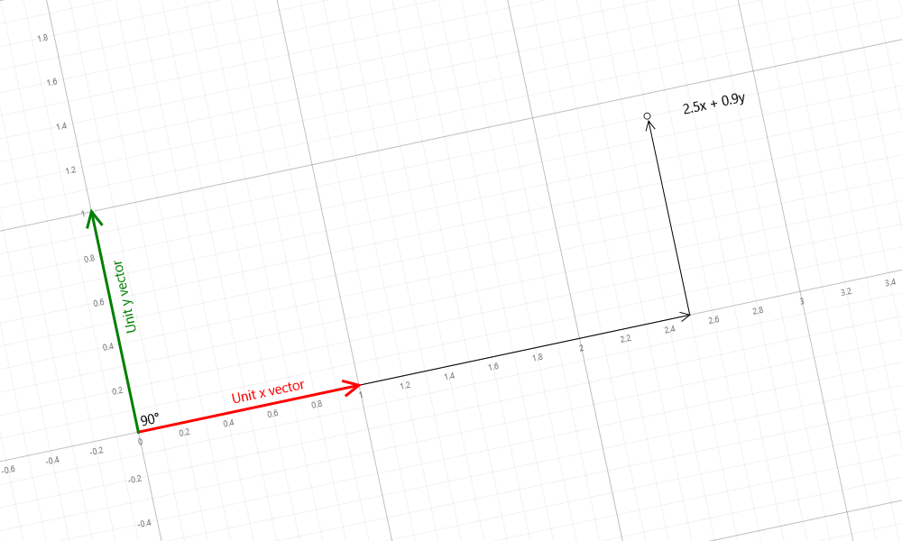
A Cartesian coordinate is a list of numbers which can be treated as multiplication factors for their respective axes as shown in Figure 2. The point specified by a coordinate is the sum of all these axis×factor pairs. For example, in a system with the axes X, Y, and Z and an origin O, the location of coordinate can be found by computing the following vector sum: .
Another benefit of Cartesian systems is their uniqueness. There is exactly one way, and only one way, to represent every finite point using a coordinate. If two points are coincident, their coordinates will be the same. If two points are different, so are their coordinates.
There are however shortcomings as well, which have led to the proposal of alternate systems. There is for example no good way to describe points at infinity using Cartesian coordinates. We are of course free to insert an infinite value into a coordinate, but this yields at most eight distinct points infinitely far away from the origin, shown in Figure 3. It doesn’t matter what the finite value is, compared to infinity it is meaningless and might as well be zero.
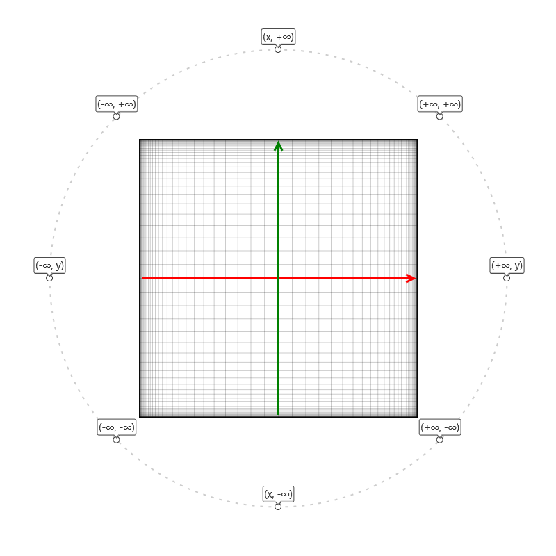
The other big drawback is that the Cartesian system is only well-behaved within a flat space. This makes it unsuitable for large scale cartography since the Earth is round, for relativistic cosmology since spacetime is curved, and for non-Euclidean geometry in general.
Incidentally, it is possible to generalise Cartesian systems to have non-perpendicular and non-unit axes. The properties and spatial coverage of these oblique coordinate systems are mathematically very similar to those of the Cartesian system. In fact one could think of Cartesian coordinates as a special case of these more general oblique coordinates, one in which a lot of the mathematics involved with complicated vector algebra happens to simplify away into nothingness.
Grasshopper supports transformations between different oblique coordinate systems through the change of basis transformation, a more complicated version of the orient transformation, which only supports the mapping of points between Cartesian systems.
Angular Systems
When it comes to mapping the Earth and the sky, angular coordinates are more suitable than Cartesian coordinates. The near spherical shape of the Earth, its near circular orbit around the Sun, and its rotating motion around the axis demand coordinate systems compatible with cyclical spaces. Cartesian coordinates work well in flat spaces which do not curve back in on themselves, but when they get crowbarred into cyclical spaces there will be seams where two adjacent points in space nevertheless have wildly differing coordinate values.
When the cyclical direction is represented not by a distance coordinate but by an angle coordinate, it more naturally tracks the structure of the underlying space. Provided at least that the angles 0°, 360°, 720°, etc. are taken to be different representations of the same angle. This is why angular systems tend not to be unique, as one can freely add multiples of a full rotation to the angular values in a coordinate without affecting the location of a point.
Another reason to use angular coordinates is when the choice of origin has great significance. Cartesian systems are all quite fungible, in that moving the origin or re-orienting the axes yields another Cartesian system every bit as good as the first. But an angular system attaches importance to the origin location since the accuracy of coordinates is higher near the origin. For example the coordinate “two days travel North-East of Rome” only makes sense when the origin of the system is a meaningful point. Nobody would care to provide directions from Rome to Florence using Helsinki as an origin point.
The most common angular systems are polar systems, which combine one or more angular values with one or more distance values. In three dimensional space two types of polar coordinate systems can be specified: cylindrical systems consisting of one angle and two distances, and spherical systems consisting of two angles and one distance.
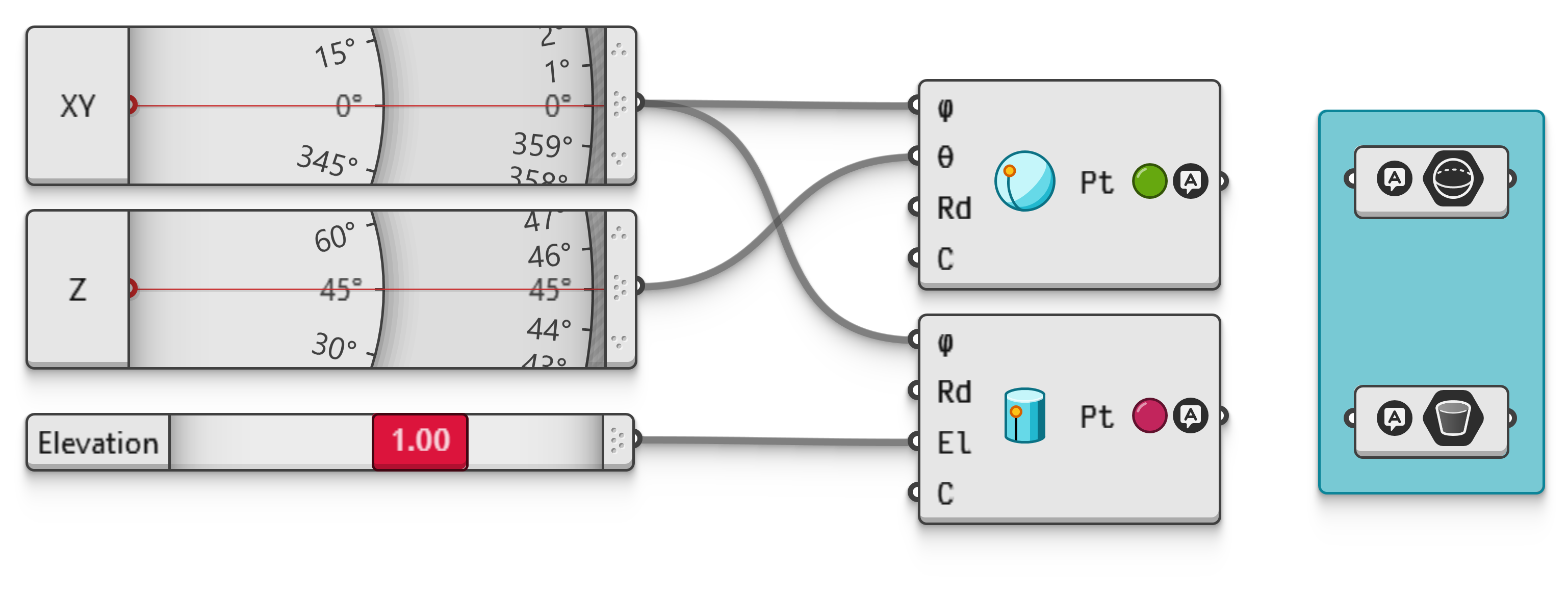 Interactive in Grasshopper 2
Cylindrical systems consist of a single angle measured in the base plane starting from the 'zero-axis', a radial distance travelled in the direction specified by this angle, and a second distance travelled perpendicularly to the base plane. Spherical systems consist of the same angle measured within the base plane, a second angle away from the base plane, and a single distance value.
Polar systems can faithfully represent points-at-infinity with coordinates like as shown in Figure 5, although it still requires the use of an infinite value, which makes using such coordinates in arithmetic very awkward.
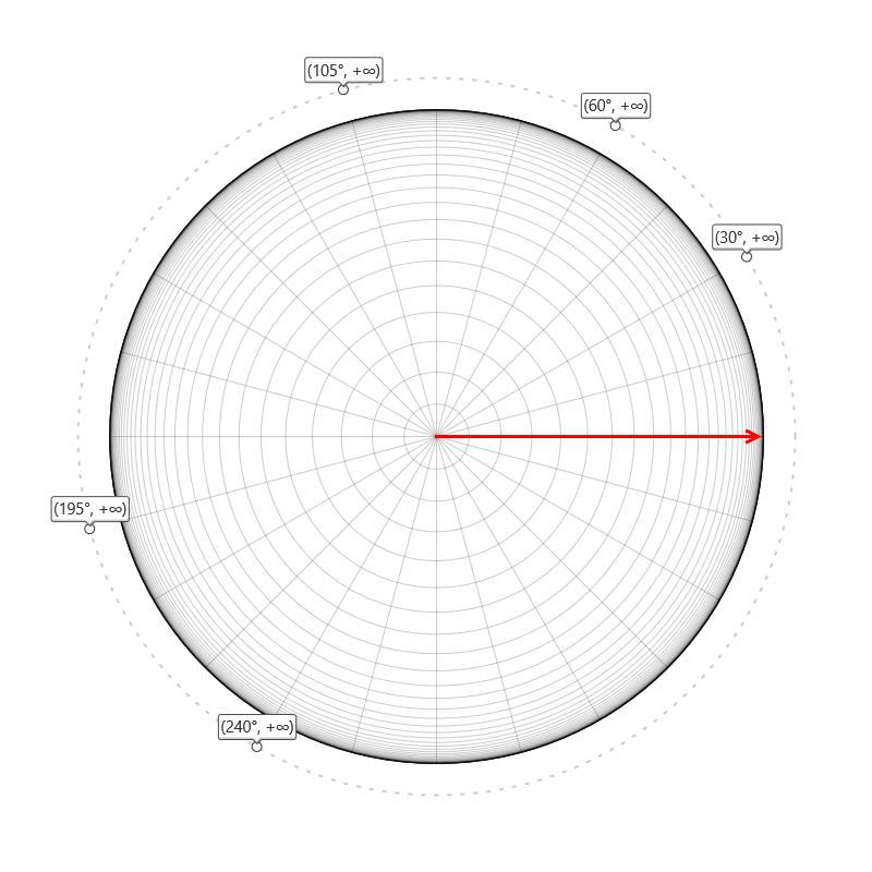
Grasshopper provides ways of creating Cartesian coordinates from various angular systems. Do note though that Rhinoceros and Grasshopper are fundamentally Cartesian platforms, so ultimately all points and vectors exist as (x,y,z) triplets.
Homogeneous Systems
In the early 19th century, August Möbius developed homogenous or barycentric systems as a way to solve the points-at-infinity problem within the Cartesian framework. The two main benefits of these systems are that they are based on —or at least compatible with— Cartesian systems, and that points infinitely far away from the origin do not require infinite values in the coordinates. Figure ?? shows what happens to a point if the w coordinate approaches zero. The downside is that a homogeneous coordinate for an n-dimensional space requires more than n components.
A typical example of a homogeneous coordinate in a three-dimensional space would be (x,y,z,w), where w is a weighting factor. The conversion to regular Cartesian coordinates would be , which means that for very small values of w the point will be very far away from the origin. When w approaches zero, the point approaches infinity, in the direction specified by the ratios of the x, y and z components.
At present there's no way to create points from homogeneous coordinates in Grasshopper, but there is a component for creating barycentric coordinates within triangles, which are a different formulation of homogeneous coordinates.
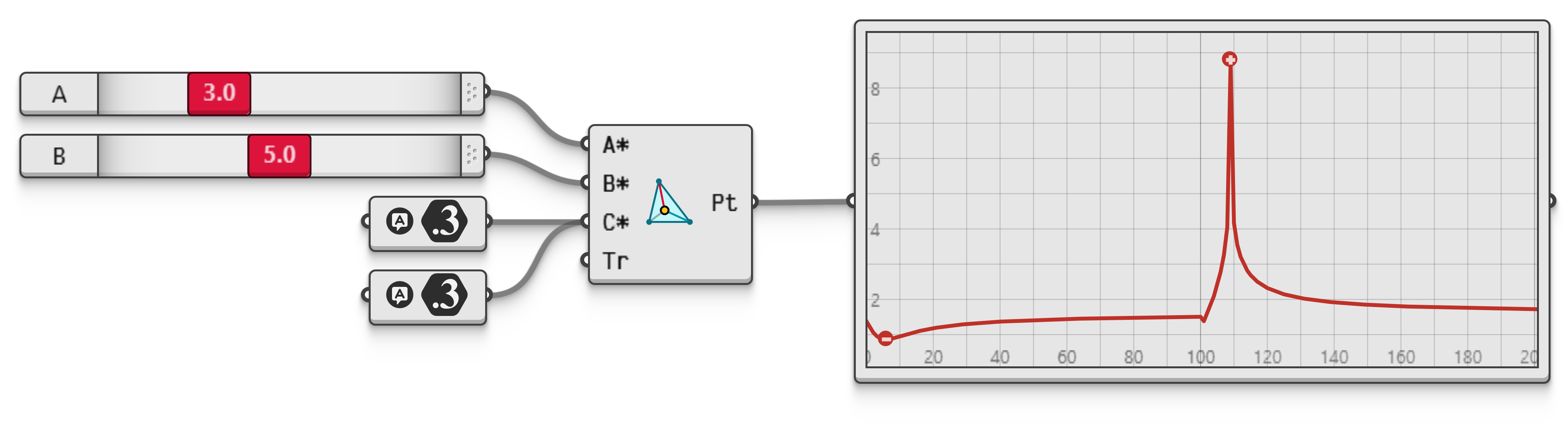 Interactive in Grasshopper 2
In Rhinoceros there are two uses for homogeneous coordinates; NURBS control points and point transformations, both of which are advanced topics discussed elsewhere in more detail. NURBS geometry supports weighted control points, meaning coordinates with three spatial values and a weighting factor. However these coordinates can usually be treated simply as a compound of a Cartesian coordinate and a weight number. The homogeneous qualities of control points only become relevant in the low level mathematics associated with NURBS shapes.
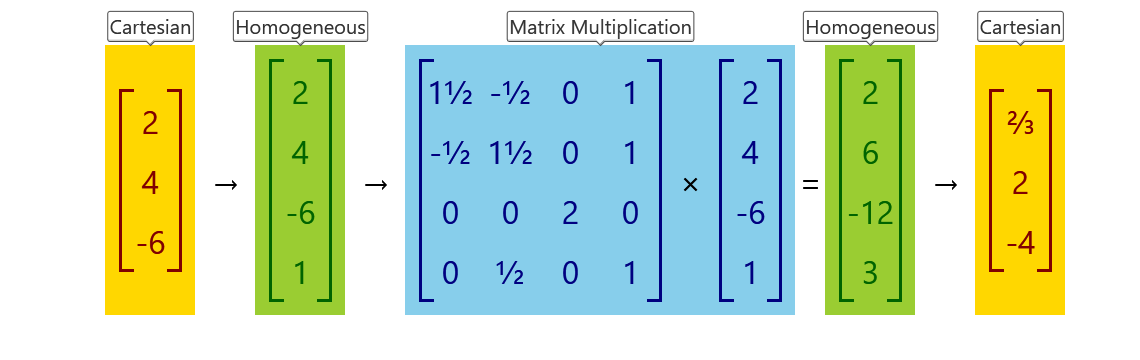
In the case of point transformations, an obvious problem is that a three-dimensional Cartesian point cannot be transformed by a transformation matrix, as matrix multiplication requires matrices with a shared row or column count. Cartesian points can be treated as a matrix, but turned into a matrix by adding a homogeneous w component with value 1.0. Finally a reverse conversion step is required in order to get the location of the transformed point in the Cartesian (x,y,z) form. Figure 7 shows the steps required to transform a Cartesian point with a matrix.
Again, as with NURBS control points, the homogeneous qualities of point transformations are completely abstracted by the Rhinoceros api and need not be taken into account unless one is writing low level code.
Fractal Systems
Where homogeneous systems sacrifice brevity in order to solve a particular problem, fractal systems can be used to reduce the number of coordinates. Fractal systems define locations in n-dimensional spaces using fewer than n coordinate values. In Grasshopper, the only fractal system available is based on the Hilbert space filling curve.
Space filling curves meander so strongly that in the limit case they manage to fill up a space with a dimension higher than 1. In effect, space filling curves lose a meaningful length property, but gain a certain kind of area property. The Hilbert curve is created by repeatedly adding smaller and smaller orthogonal wriggles to the Hilbert base curve until after an infinite amount of such alterations it achieves an infinite length and an area of one square unit. Figure 8 shows the first few iterations of the infinite process which, ultimately, is supposed to generate the true Hilbert curve.
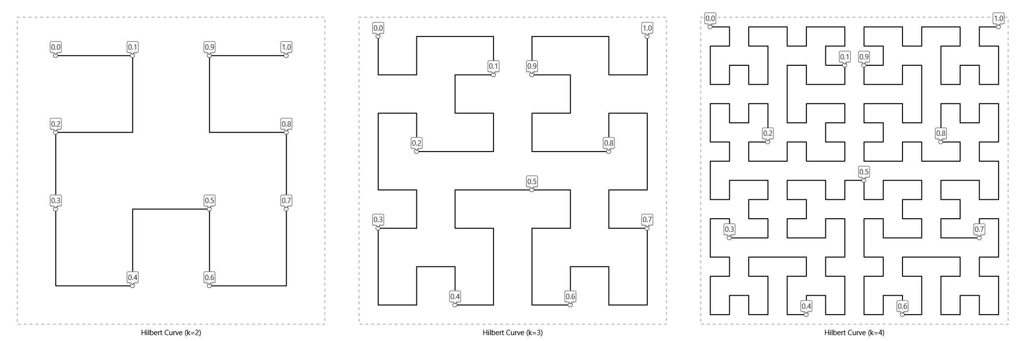
At this point, every location inside the unit square can be represented as a Cartesian (x,y) coordinate, or as a length proportion along the Hilbert curve. There thus exists a mapping from a bounded two-dimensional space (the unit square) to a bounded one-dimensional space (the unit domain). In reality, it is not possible to generate a true Hilbert curve, as it would require an infinite amount of computational steps to do so. Instead, a sufficiently accurate intermediate curve is used.
The benefit of the Hilbert curve over other fractal approaches is that is has excellent locality preservation. That is, points which are close together in 2D space will also often be close together in Hilbert space, although it is not mathematically possible for this to be true of all pairs of nearby points.
Conclusion
Coordinate systems are everywhere in 2D and 3D modeling applications. Points must be written down as some sort of coordinate, and those coordinates only make sense in the context of a specific coordinate system. Rhinoceros and Grasshopper both operate using a privileged Cartesian system called World XY, but it is possible to define points and transformations using other coordinate systems. Without a solid understanding of the various types of coordinate system along with their applicabilities and limitations, professional results become a fool's errand.