The cursor can always move freely, but sometimes you may need to put some restrictions on the cursor. You can restrict the cursor’s movement to the CPlane Grid , to a distance or angle, snap to existing objects, or enter coordinates to locate points in space.

The Rhino Cursor

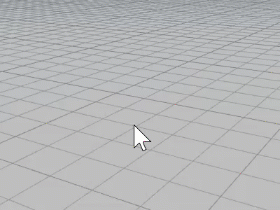
The Rhino cursor 1 consists of a marker 2 and a cross 3 . The marker usually stays at the center of the cross. The cross always follows the mouse movement. The marker becomes available when running a command that requires picking points.

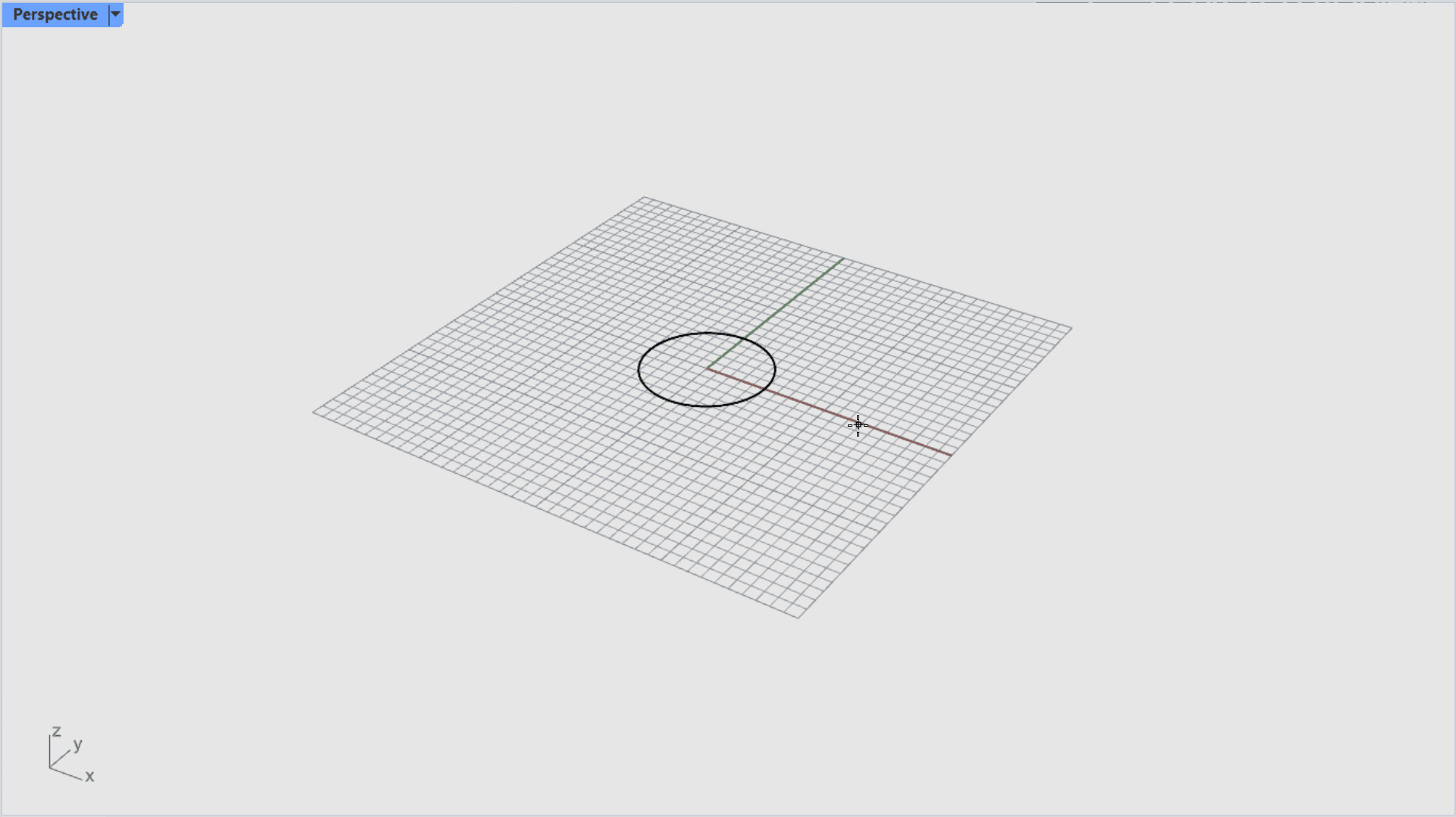
The marker may leave the cross when a constraint is in effect. For example, when Elevator mode is active, a tracking line connected to the marker displays. The location of the marker is picked when you click the left mouse button.

Construction Plane

The Construction Plane or CPlane determines how geometry is placed in space. It’s responsible for both its location and orientation. It is visually represented by the Grid , yet extends infinitely beyond it.

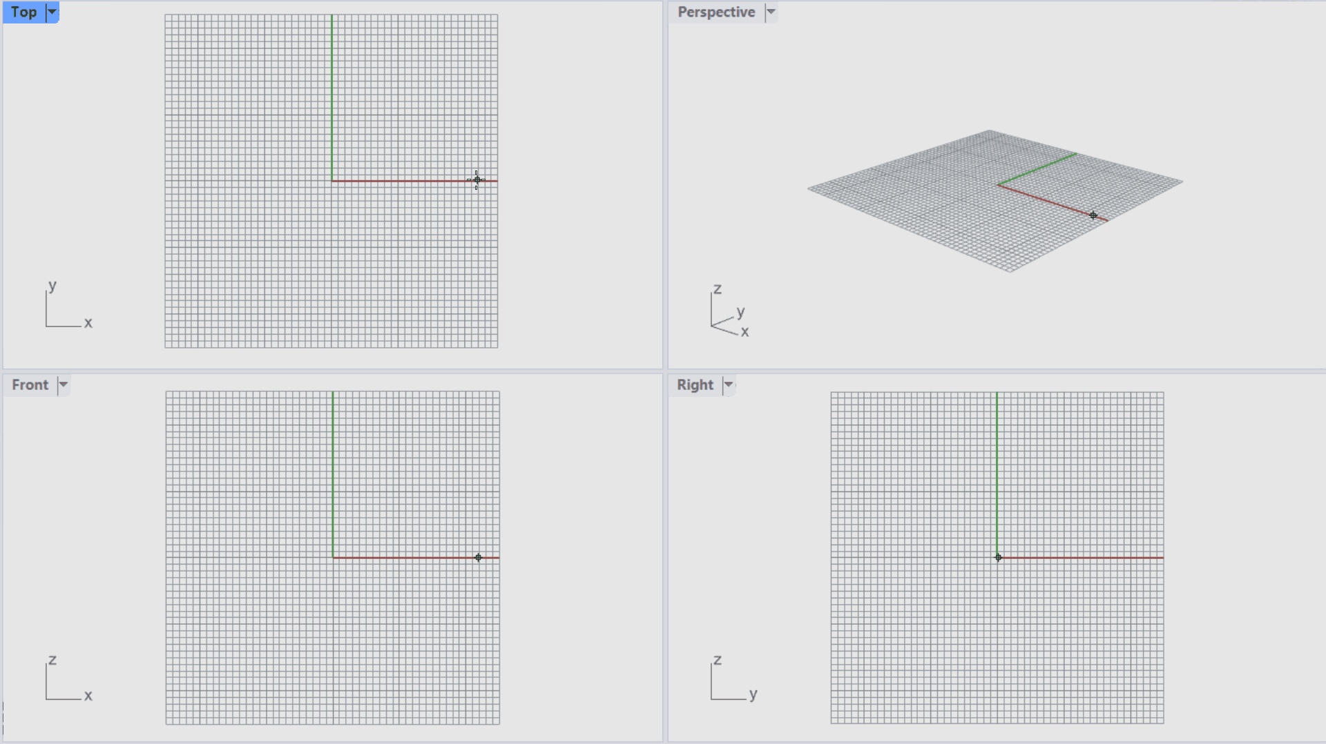
Each Viewport has its own Grid orientation. The Perspective and Top share the same Grid

The AutoAlignCPlane allows to easily orient the CPlane to a planar object, such as a curve or surface. This automatic way of setting a CPlane lets you draw on a face of an object.

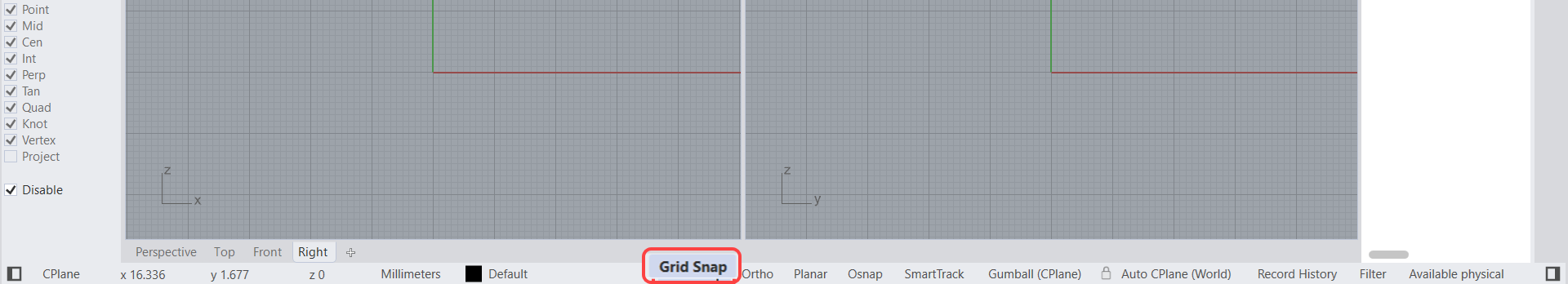
Grid Snap

Grid Snap constrains the marker to the crossing points of the Grid that extends infinitely in the X and Y directions. It is useful to place points and draw segments aligned at precise intervals.

Click the Grid Snap pane on the Status Bar to turn it on and off or press F8 . Right-click the Grid Snap pane to change its Settings.

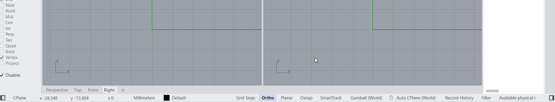
Ortho Mode

Ortho constrains the marker movement to a specific angle. By default, it’s 90ª and parallel to the grid lines.

Click the Ortho pane on the Status Bar to turn it on and off. Hold the Shift key to temporarily toggle Ortho . Right-click to change its Settings.

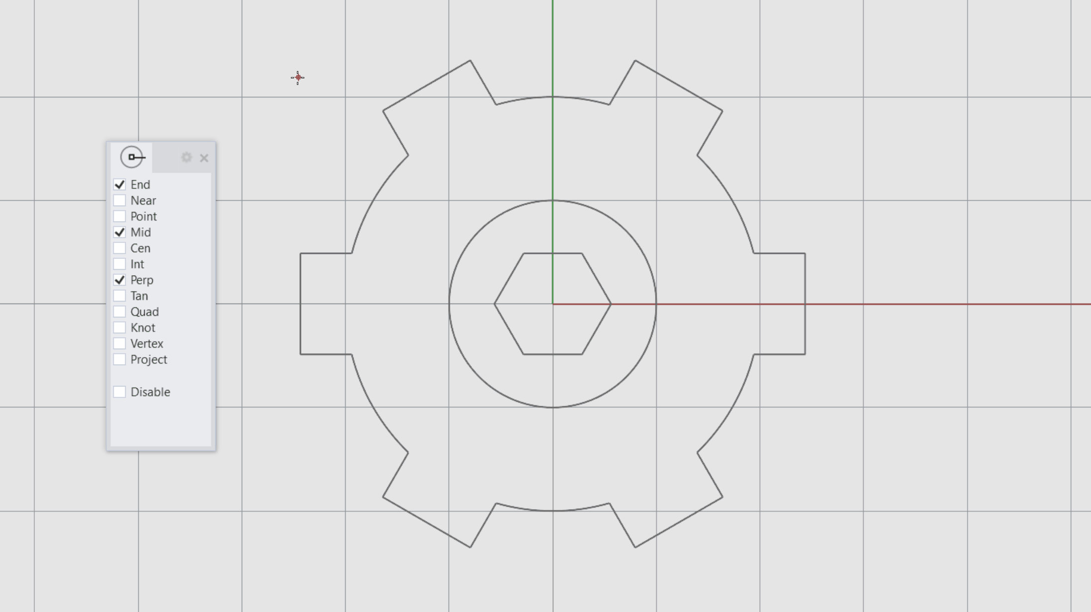
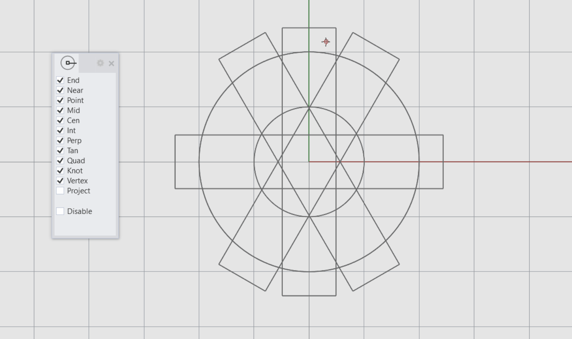
Object Snaps

When Rhino asks you to pick a point (eg: start of a line), object snaps allow you to pick a precise location on an existing object. When you move the cursor near that location the marker jumps to it.

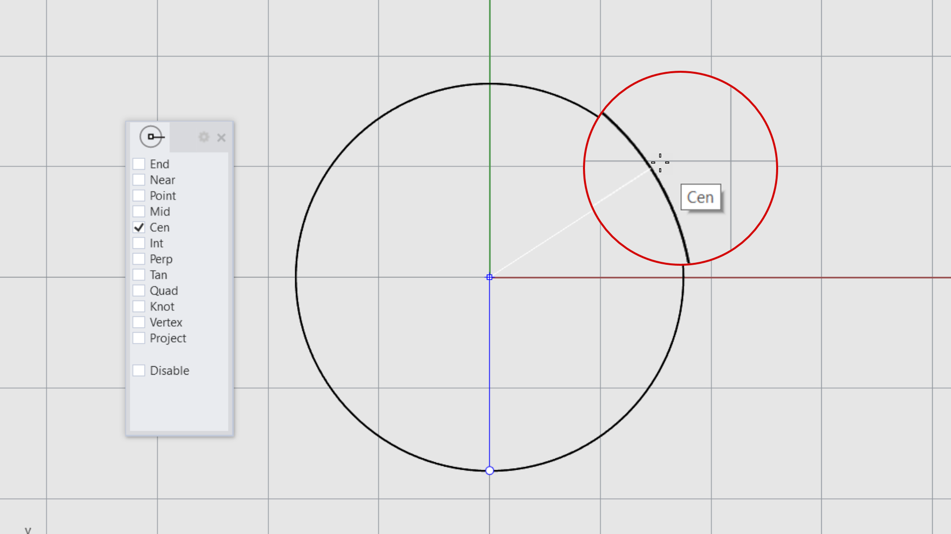
Osnap Control

Object Snaps are set in the Osnap Control . It is docked at the bottom left of the screen. It can be docked at other locations or floated.

Persistent Osnaps

Persistent Osnaps are the ones selected in the Osnap Control . Once selected, they will be active anytime you reference that point on an existing object.

Osnap Functions

• To temporarily deactivate Osnaps: Hold down the Alt key.
• To disable Osnaps: Select Disable in the Osnap Control .
• To clear all Osnaps: Right-click on Disable in the Osnap Control .
• To select one Osnap: Right-click on one Osnap in the Osnap Control . It will clear all others from selection.

One-Time Osnaps

Multiple persistent object snaps may interfere with one another, so you can also turn on an object snap for a single pick. One-time object snaps override persistent object snaps. This lets you keep your persistent object snaps set, but to override them for the next pick.

To activate them, hold down the Shift key and select the object snap in the Osnap Control .

Or access them through the Osnap Toolbar

Complex Osnaps

Some special object snaps let you select multiple reference points or add advanced references. See the Object Snaps Using References topic.

Complex Osnaps are available from the Osnap Control while pressing the Ctrl key.

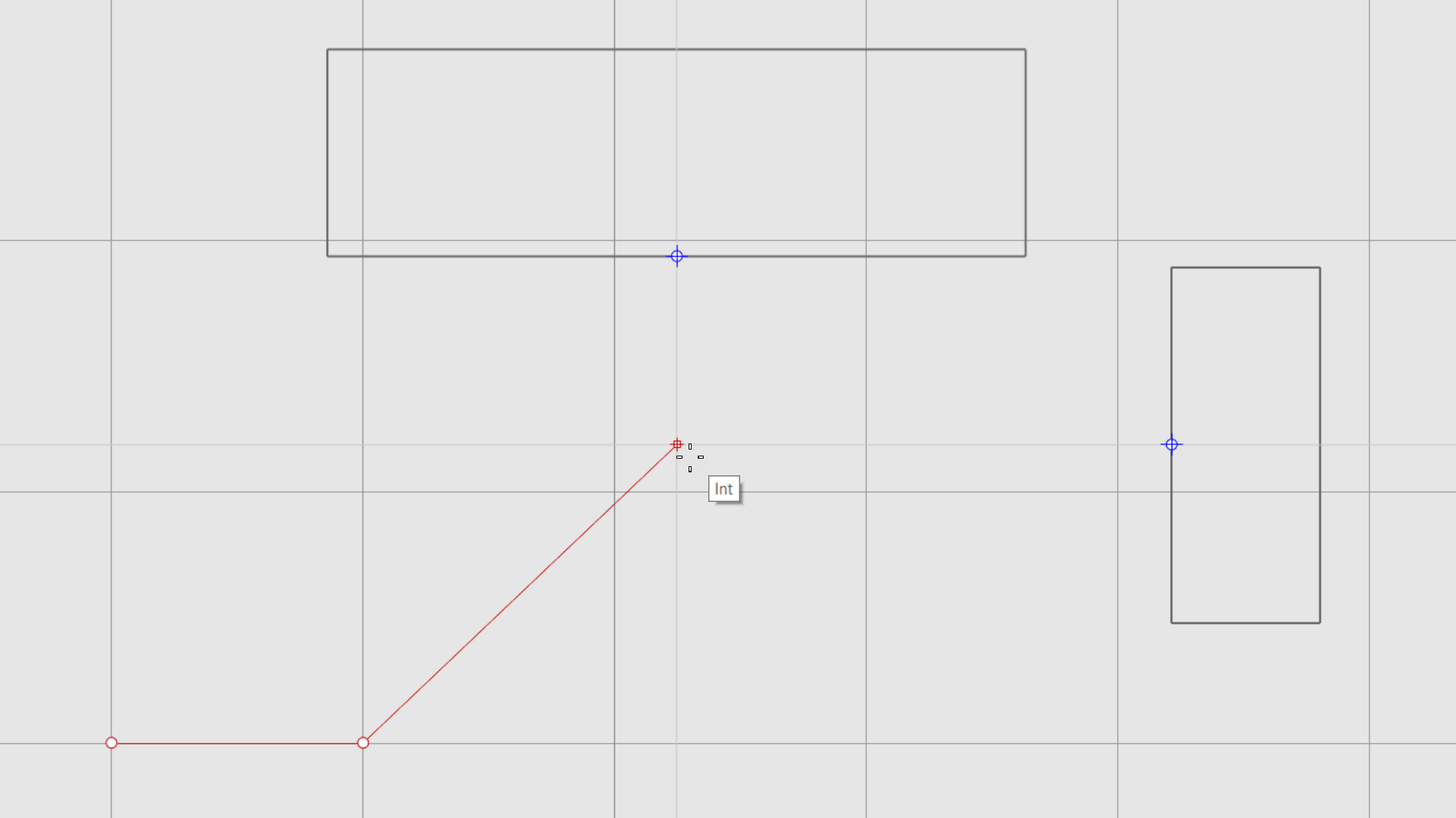
Distance & Angle Constraints

When entering points, you can restrict the cursor to a distance or angle from the previous point. An easy way to achieve this is using Grid Snap or Ortho . If you need to enter a different distance or angle value, you can use Distance or Angle Constraints.

Distance Constraint

The distance constraint restricts the distance the cursor can travel from the previous point.

To set the distance during a command type a number in the Command Prompt . This value is updated when typing a new number before placing a point.

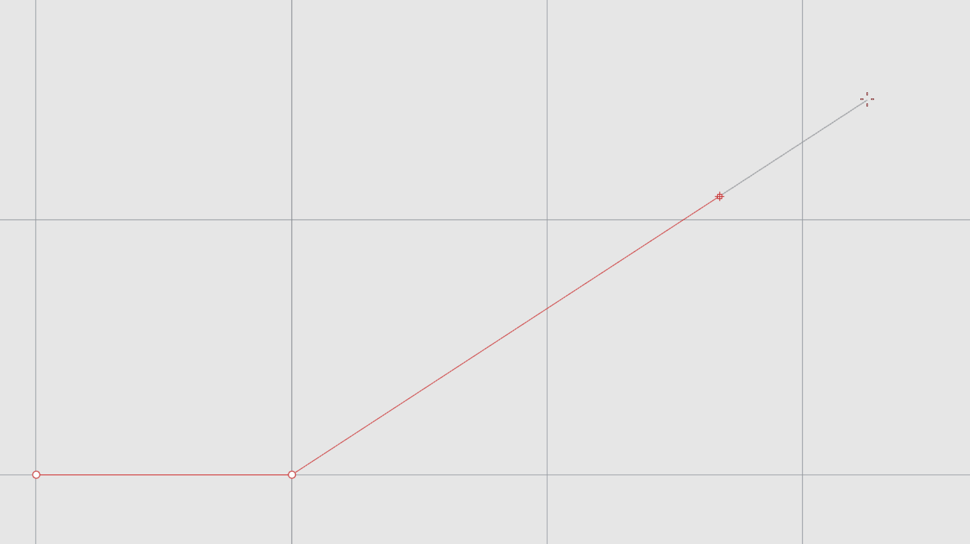
Angle Constraint

Angle constraint is similar to Ortho , but you can set any angle. The angle is only in effect for the next pick.

To set the angle during a command type < sign followed by the angle value in the Command Prompt . The smaller than sign tells Rhino it’s an angle.

To use Distance and Angle constraint together:

1. Open a New file.
2. Select your Template of choice.
3. Run the Line command.
4. At the Start of line prompt, type 0 and press Enter .
5. At the End of line prompt, type 10 for a distance of 10 units.
6. At the End of line prompt, type <35. This sets the angle every 35º.
7. Click in the view to set the end point at the first 35º.

SmartTrack

SmartTrack is a system of temporary reference lines and points drawn in the viewport. It uses implicit relationships among 3‑D points, geometry, and the coordinate axes directions.

Tracking lines and smart points can be used by object snaps just like real lines and points.

You can snap to intersections of tracking lines, perpendiculars, smart points and real curves. The tracking lines and smart points are displayed only for the duration of a command.

Click on the SmartTrack pane on the Status Bar to turn it on and off. Right-click to change its Settings.

Coordinate System

Rhino uses two coordinate systems: construction plane coordinates and world coordinates. Construction plane coordinates are defined for each viewport. World coordinates are fixed in 3‑D space. Details on coordinate systems…

Right-Hand Rule

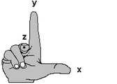
Coordinate systems follow what is called the right-hand rule. The right-hand rule can help you determine the direction of the z‑axis in a coordinate system. Form a right angle with the thumb and forefinger of your right hand. When your thumb points in the positive x‑direction, your forefinger points in the positive y‑direction, and the palm of your hand faces in the positive z‑direction.

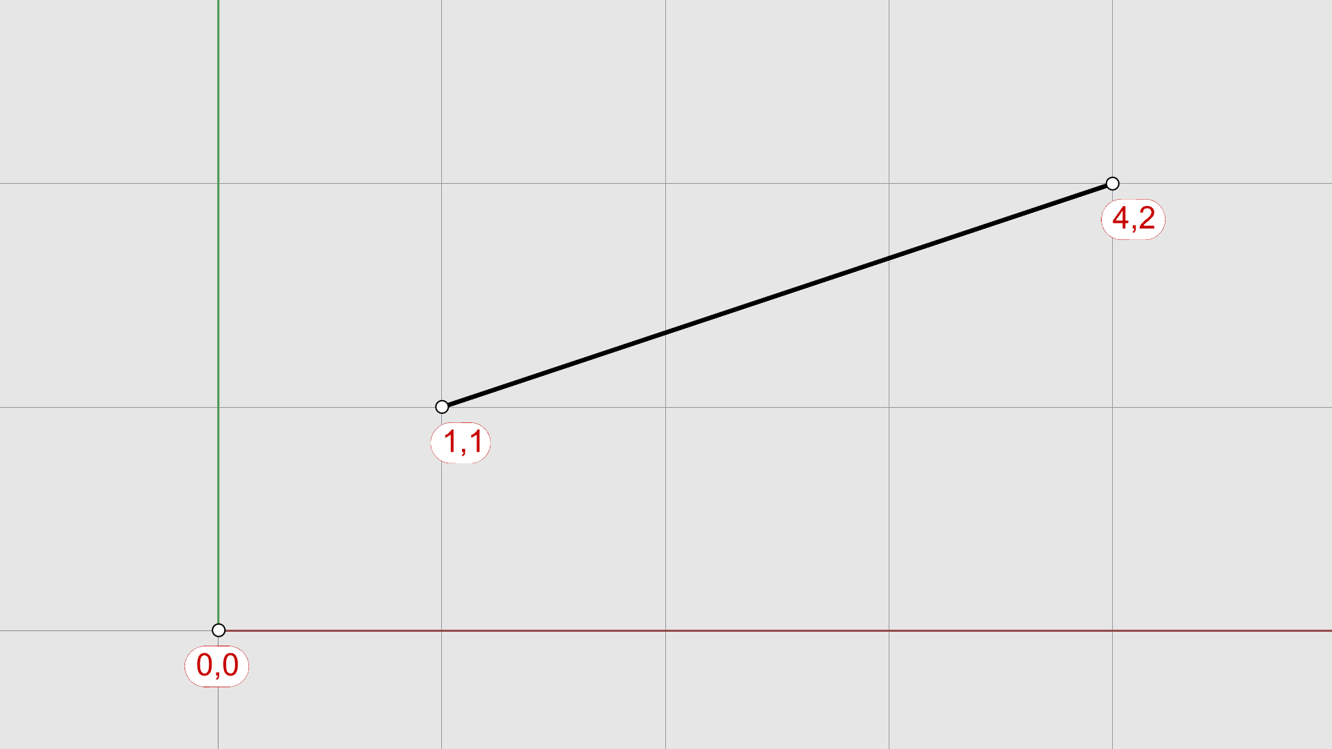
CPlane Coordinate Entry

One way to enter points at precise locations is using coordinate entry. Rhino understands CPlane, World and Relative coordinates.

To enter CPlane coordinates:

1. Open a New file.
2. Select your Template of choice.
3. Run the Line command.
4. At the Start of line prompt, type 1,1 and press Enter .
5. At the End of line prompt, type 4,2.

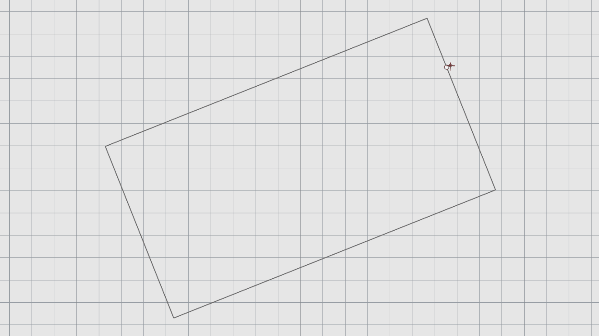
Elevator Mode

Elevator Mode lets you pick points that are off the construction plane in the positive or negative Z‑direction. You can activate it by holding the Ctrl / CMD and clicking a point on the CPlane .

To use Elevator Mode:

1. Open a New file.
2. Start the Polyline command.
3. Pick a first point on the CPlane and drag away.
4. Press the Ctrl / CMD key while you pick a second point.
5. Enter a value in the Command Prompt or pick a point to set the height.

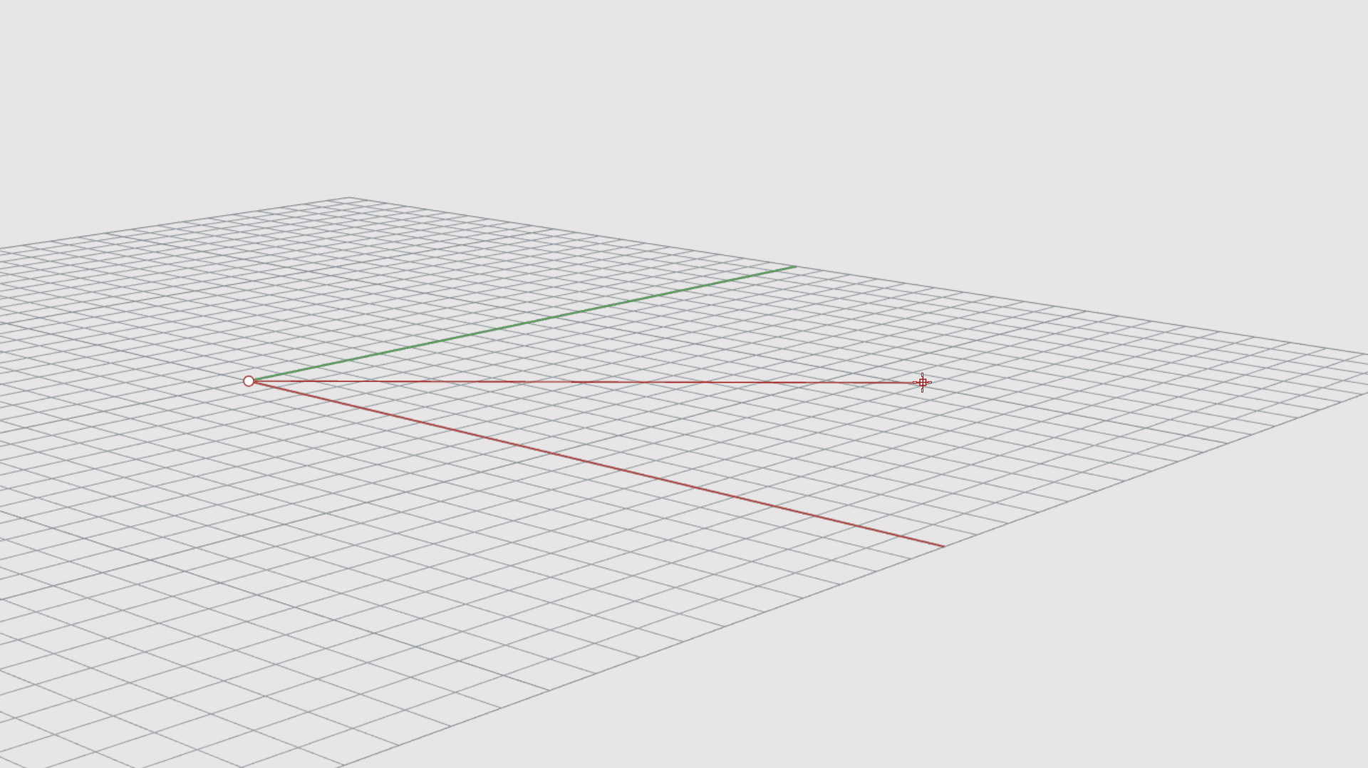
Using elevator mode to move your pick point vertically from the construction plane lets you work in the Perspective viewport more easily.

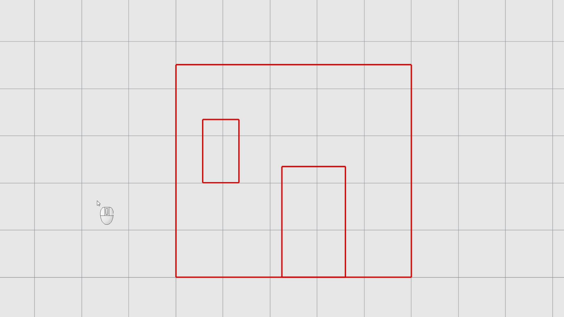
Direction Lock

After placing a first point, Direction Lock allows you to reference a point and locks the cursor’s trajectory to it. You can activate it, by holding down the Tab key.

To use Direction Lock:

1. Open direction-lock.3dm in Rhino
2. Run the Polyline command.
3. Activate Near and Perp OSnaps in the Osnap Control
4. Pick a point on the Rectangle using the Near Osnap.
5. Approach the cursor to the opposite side until you see the Perp OSnap. Press the Tab key.
6. Enter a value in the Command Prompt or pick a point in the view to set the actual length.

Gumball

The Gumball is a widget with handles to easily Move , Rotate , Scale and Copy objects in Rhino. You can do this freely by manipulating the different handles.

Click the Gumball pane on the Status Bar to activate it. Now, it will be visible anytime you select an object(s).

Transforming with Units

Click on any of the Gumball handles to access the numeric entry box. Type a value to apply a distance, angle or scale factor of your choice.

Snappy Dragging

The Gumball pays attention to Osnaps when set to Snappy Dragging. This will allow you to snap and align objects together with precision.

To set Snappy Dragging, Right-click the Gumball pane on the Status Bar and select Snappy Dragging.

Relocation

Double-click on any of the Gumball Handles to reposition it elsewhere on the object. All modifications happen from the Origin of the Gumball . Notice how this affects the result…

To reset the Gumball’s default orientation and location, right-click the Gumball pane on the Status Bar and select Reset Gumball.

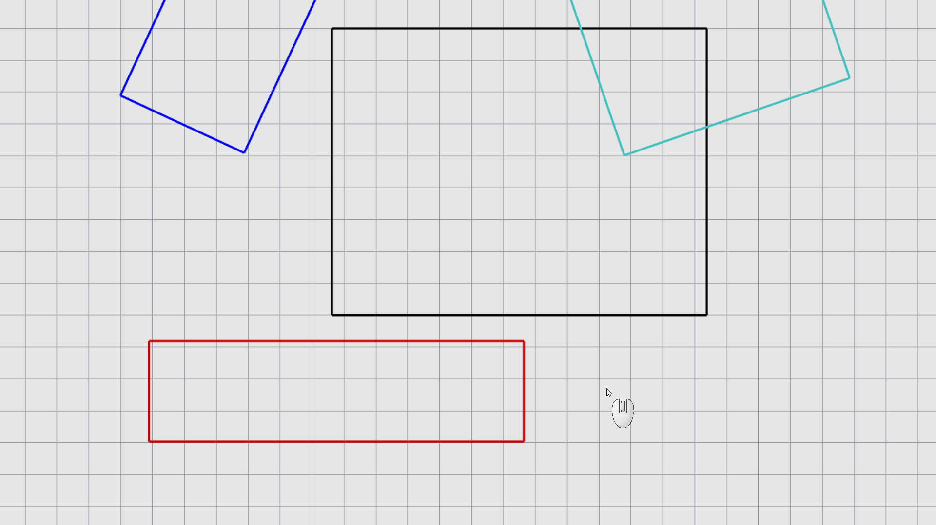
Exercise 1: Move Objects

In this simple exercise, learn how to use the Gumball to move an object to a specific reference point.

1. Open first-gumball-exercise.3dm in Rhino . Welcome to Tetris!
2. Activate the Gumball .
3. Right-click the Gumball pane on the Status Bar and set it to Snappy Dragging.
4. Select only End and Near from the Osnap Control
5. Select the red rectangle.
6. Double-click the Gumball plane. This will activate relocation. Snap it to the bottom-left corner.
7. Drag the red rectangle using the Gumball plane, to the bottom-left corner of the black rectangle.

Exercise 2: Align Objects

In this simple exercise, learn how to use the Gumball to align an object to two reference points.

1. We’ll use the same file and Gumball settings as above.
2. Select the blue rectangle.
3. Double-click the Gumball plane. Snap it to its bottom-left corner.
4. Double-click the Gumball arc. Snap it to the bottom-right corner.
5. Drag the blue rectangle using the Gumball plane, to the top-left corner of the red rectangle.
6. Rotate the blue rectangle using the Gumball arc, until it’s aligned with the top edge of the red rectangle. Use End or Near OSnaps as a reference.

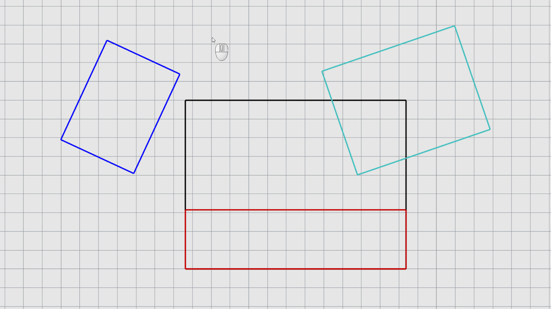
1. Try it on your own! We are leaving the cyan rectangle for you to place it in position.

Learn More

---

Edit this page

Edit on GitHub

History

Admin