The continuity between surface edge pairs can be analysed with
![]() EdgeContinuity
.
EdgeContinuity
.
When you want to analyse a large number of edge pairs however,
![]() GlobalEdgeContinuity
helps to get a quick overview of the continuity between surfaces in your model.
GlobalEdgeContinuity
helps to get a quick overview of the continuity between surfaces in your model.
GlobalEdgeContinuity evaluates continuity between surfaces for G0, G1 and G2. The surfaces can, but don’t need to be joined. In fact, the preferred way is to not join any surfaces during modeling. Edge matching is done automatically after selecting the surfaces to evaluate.
Single or Multiple
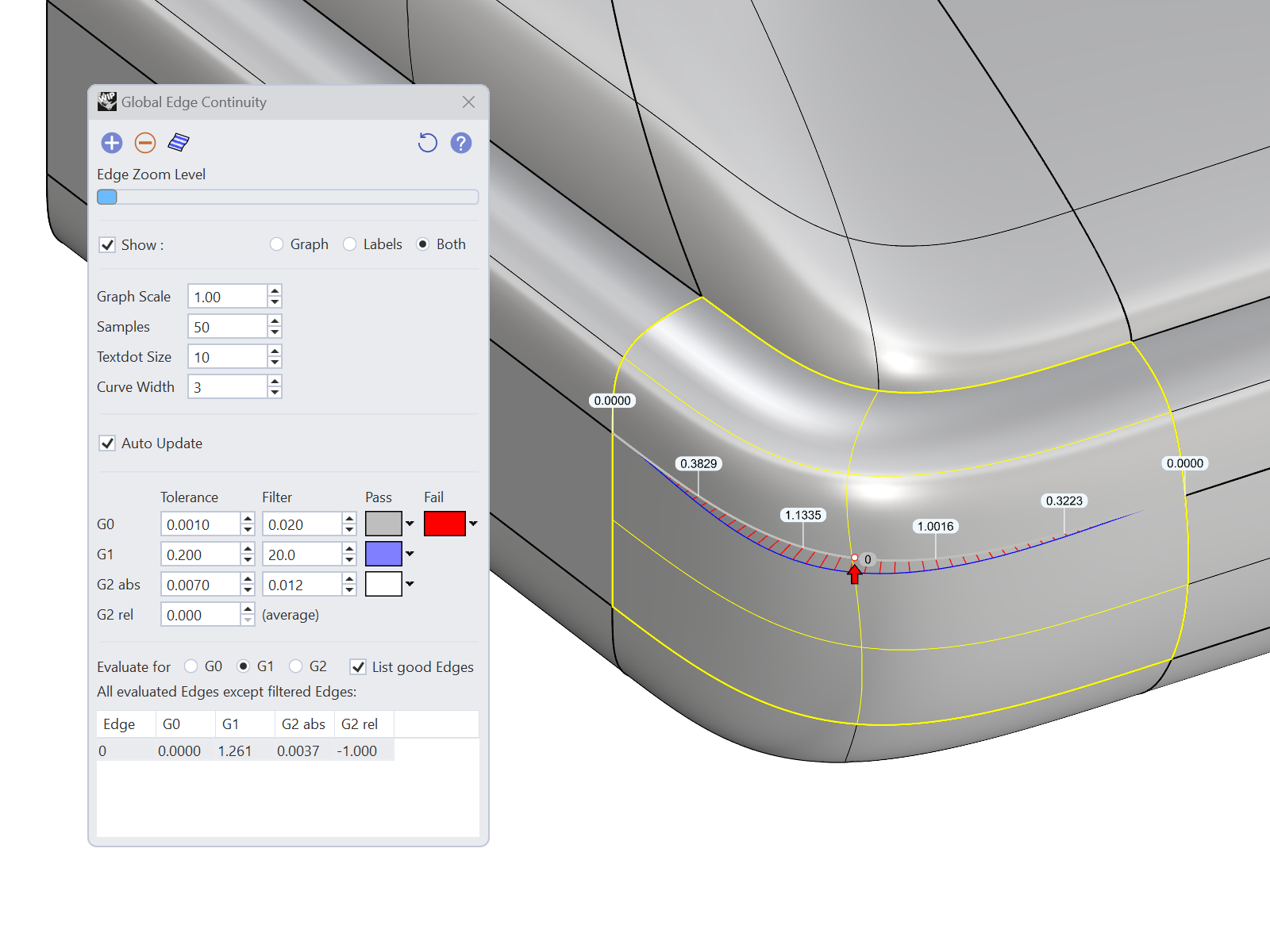
When selecting only one surface, its direct surrounding surfaces will be found automatically. Only the edges of the selected surface will be evaluated:
When selecting two or more surfaces, only those surfaces will be considered in the analysis:
User Interface
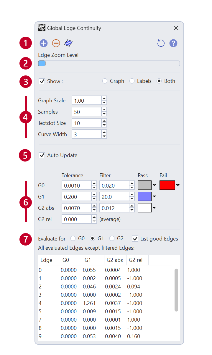
1 Top row buttons
The top row buttons in order of appearance:
On the left:
- Add surfaces to the evaluation
- Remove surfaces from the evaluation
- Zebra: opens or closes the Zebra analysis panel, and adds the surfaces in the evaluation to it.
On the right:
- Reset to defaults: loads defaults for all the settings. Any changes made are automatically stored in your Rhino settings.
- Online help
- Toggle Analysis disply on/off
2 Display
You can show and hide labels.
a only labels
b only graphs
c both labels and graphs
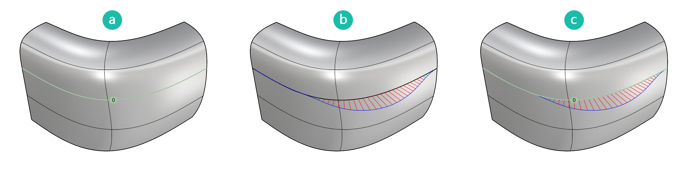
Edges are numbered and their number can be found back in the table. The graph shows a visual representation of the deviation along the edge. Note that this is not a curvature graph. Parts of the edge that are out of tolerance will be displayed red, and parts that are within tolerance will be displayed green. Use this information to add detail or manipulate controlpoints in the area where adjustment is needed.
3 Evaluate
Here you can select if you want to evaluate for G0, G1 or G2 continuity between surfaces. If G0 is selected, edges that are out of tolerance will show up red. Edges that are within G0 tolerance are shown in Gray. Higher level edges are shown in blue when they meet G0 and G1 tolerance, or in white if they meet G0, G1 and G2 tolerance.
The recommended workflow is to work from left to right, starting with G0 analysis. Once all edge pairs meet the G0 tolerance, proceed to the next continuity level G1. In this stage, edges that are within tolerance will light up blue. The edges that are out of tolerance will stay gray and show up in the table.
Finally, if you want to match for G2, change the radio button to G2. Any edges that are within the G2 absolute tolerance will be marked white. Any edges that are G1 show up blue, until they are within the defined G2 tolerance.
4 Display settings
-
Graph Scale sets the height of the deviation graph lines. The graph only shows relative difference. It doesn’t indicate the direction of the deviation. The graph is displayed on both sides of the surfaces, so that it is visible in shaded mode at all times.
-
Samples represents the amount of samples per surface edge pair. By default, 50 samples are taken for each edge pair. When focussing on a single edge pair, an indicator will be shown every 10 samples. This means an edge by default has 6 indicators when it is selected. (see edge selection in the table section of this guide)
-
Textdot Size affects the size of the labels/dots (numbered edges and deviation textdots)
-
Curve Width sets the edge overlay width in pixels. The edge overlays shows if an edge meets G0, G1, or G2 condition. The default is 3 pixels.
5 Evaluation settings
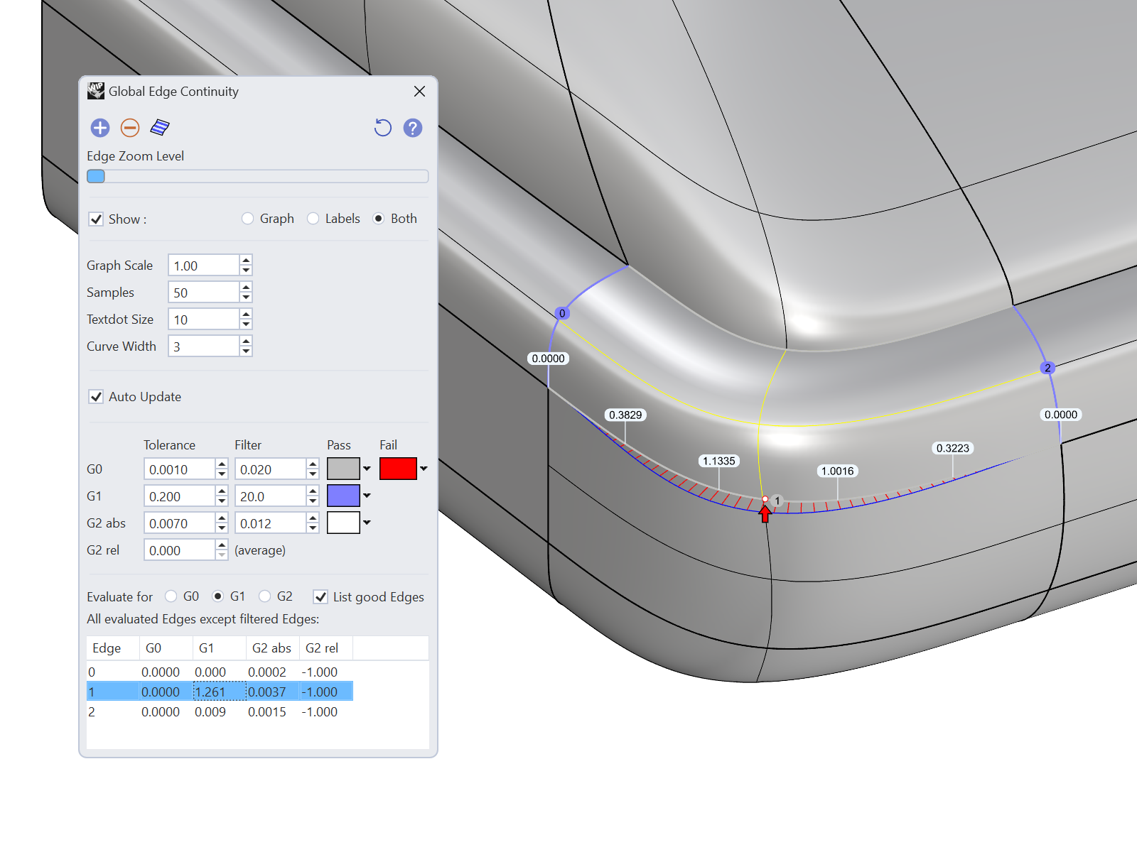
When an edge has been selected in the table, the zoom slider zooms in on the point with the highest deviation. Depending on the mode (G0, G1, G2) the point of max. deviation can be on a different location along the edge.
The UI has four different colors to indicate the state of an edge. These colors can be customized. The colors can help you quickly find edges that don’t meet your set tolerances.
-
G0 fail If an edge pair is out of positional tolerance, it means it cannot be joined. This makes the model ‘fail’ since you cannot get a watertight object. Edge pairs that are out of positional tolerance will be marked red.
-
G0 tolerance G0 tolerance, or Positional tolerance in model units. The default value is 0.001. If an edge pair is within the set G0 tolerance, it gets assigned a gray color to indicate it is joinable. The edges are considered positionally continuous.
-
G0 filter Edges that are farther apart than this tolerance are discarded from the evaluation. Adjusting this value will need a recalulation, because the value is used in the edge matching algorithm. Keep this value as small as possible.
-
G1 tolerance G1 tolerance or Tangency tolerance in degrees. The default value is 0.2 degrees. The G1 tolerance is the tolerance for edge pairs to be considered tangentially continuous. The tolerance you need is dependent on the chosen production method, as well as on subsequent steps. For example, if you are going to use the surfaces as a base for offset surfaces, any angle between the surfaces will either lead to a gap or an intersection between the offset surfaces. Once an edge has passed the G1 tolerance test, it gets the G1 color.
-
G1 filter is the maximum edge angle to evaluate. If you have intentional sharp edges, you don’t want these to show up in the list of edges that need attention. For example, a 90 degree angle is most likely intended, and with the max setting you can filter out edges that you don’t want to include in the search for ‘faulty’ G1 edges.
-
G2 abs tolerance G2 absolute tolerance or Absolute Curvature tolerance. Note that this value is scale dependent. If you scale up the model, the absolute difference decreases, and if you scale the model down, it increases. The relative tolerance is size independent.
-
G2 rel tolerance G2 relative tolerance or Relative Curvature tolerance. In some cases the avarage relative curvature can be used as a way to test for G2 continuity.
The formulae for calculating the curvature differences is:
G2 abs = (1 / r1) - (1 / r2)
G2 rel = (r1 - r2) / (r1 + r2)
Where r1 is the radius of curvature on surface 1, and r2 is the radius of curvature of surface 2. Note that these radii are signed. What this means is that one of the radii can have a negative value, if the curvature changes direction. The relative curvature difference becomes important when the directions of the curvatures don’t match (e.g. one surface curves up, and the other curves down.) In that case the relative curvature can become -1.
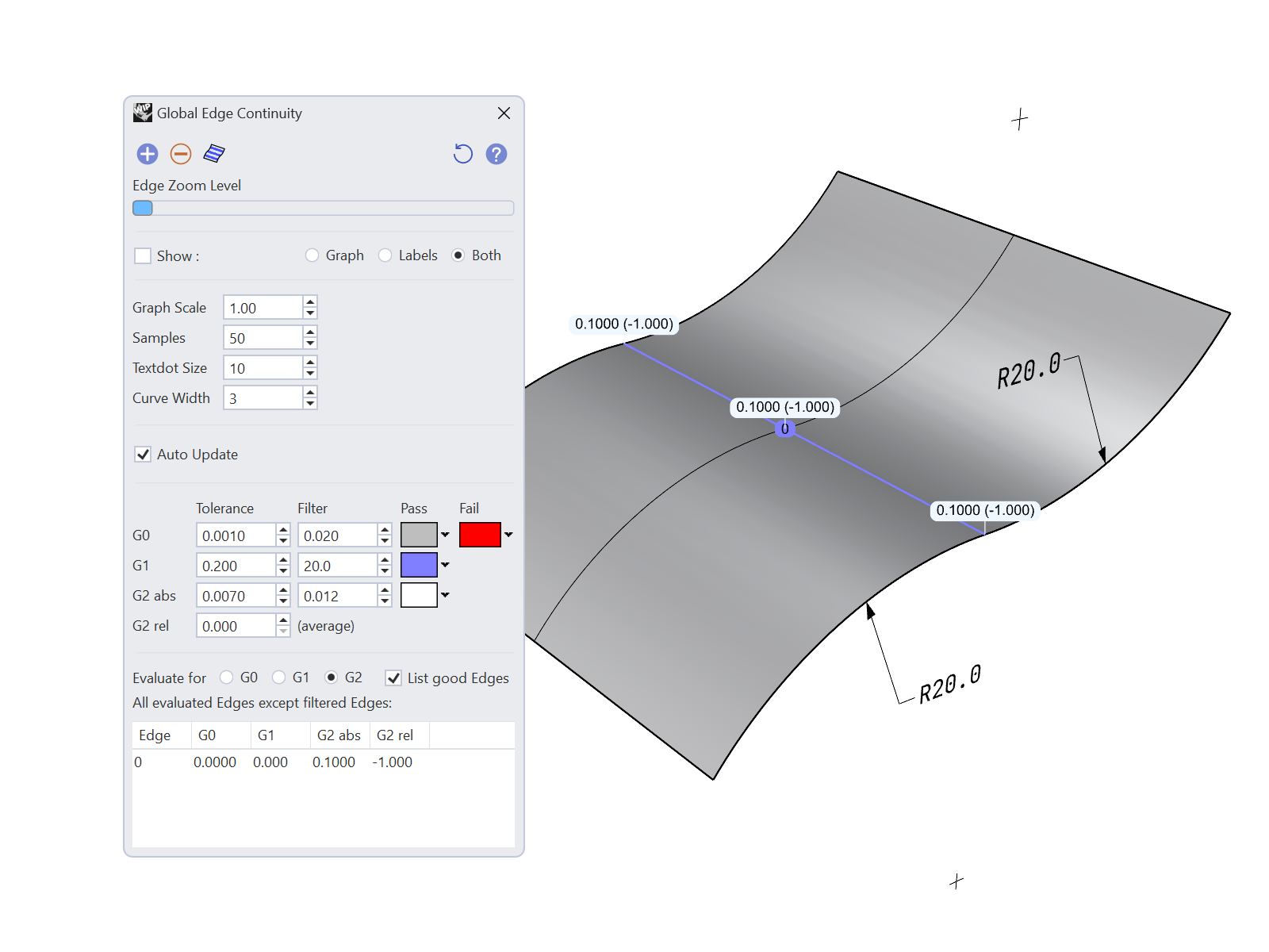
In the following image, notice that the absolute curvature difference becomes 0.1, even though the radii of curvature for both surfaces are the same, since 1/20 - 1/-20 = 1/10.
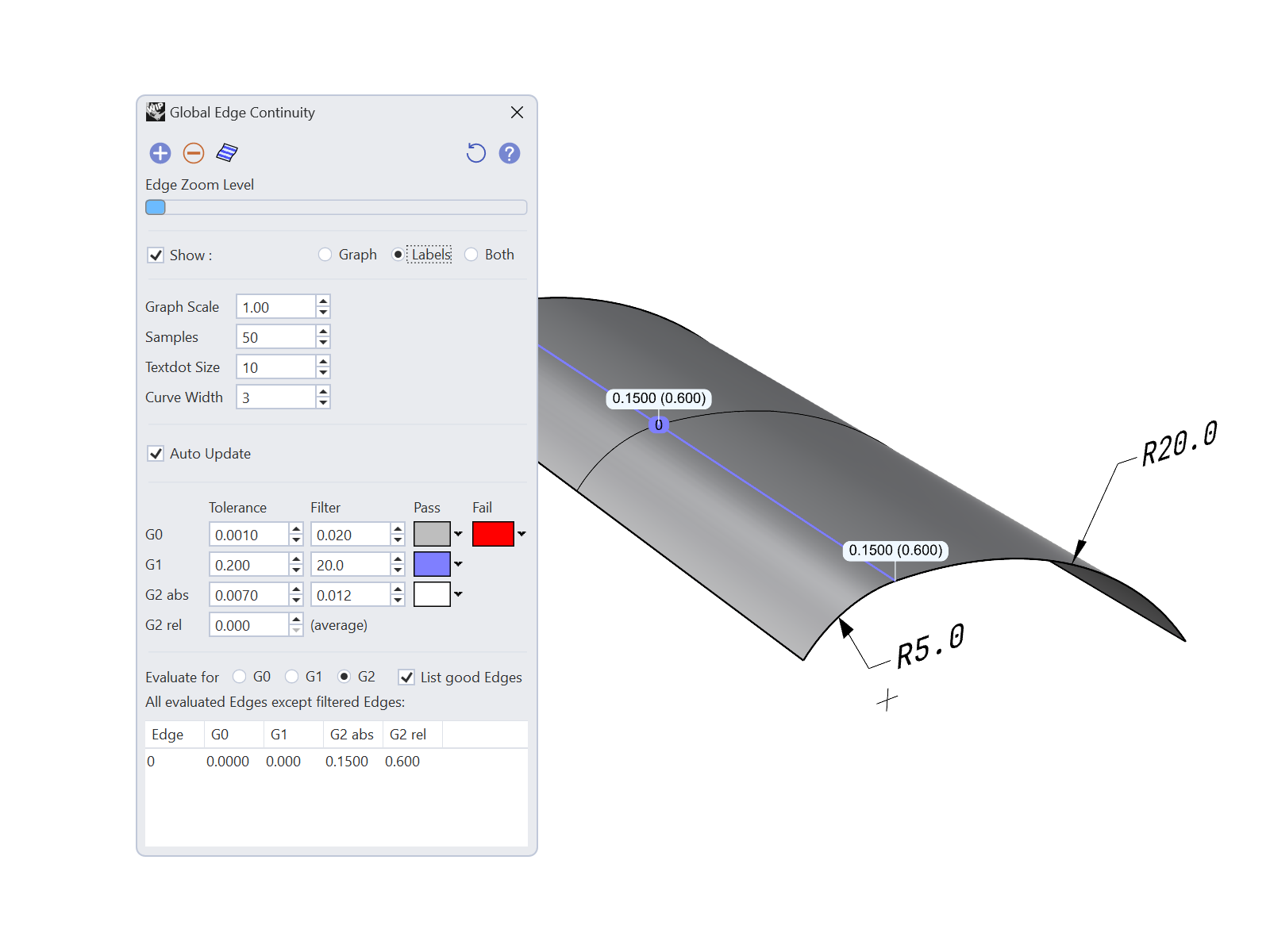
- G2 abs filter is the maximum absolute curvature difference to evaluate. This is useful to ignore surfaces that are meant to be G1 continous only. A good example of this is a G1 fillet. Since the differences in curvature are generally high, these edges can be left out from the evaluation table. A surface that has radius of curvature at the edge of 20, that connects to a fillet that has a radius of curvature of 5, will result in an absolute tolerance of 1/5 - 1/20 = 0.15 and in a relative tolerance of (20-5)/(20+5) = 0.6
6 Analysis Results
- Show Good Edges This toggle allows you to show or hide edges that are within tolerance.
-
Show Filtered G1 and G2 Edges This toggle allows you to show or hide edges that are within the filter. Note that edges outside G0 filter are discarded from the evaluation and will not be displayed, even when this option is on.
-
Zoomlevel for Selected Edge If you select one of the edges in the table, this slider allows you to zoom into the edge. The center of zoom is the point of highest deviation.
7 Results Table
The analysis results are displayed in a table. To see which edges need adjustment, leave “Show Good Edges” off. If the table shows no items, it means that all edges are within tolerance (or they exceed the G0 filter value)
Sorting of results The edges listed in the table can be sorted based on label number, G0, G1, and G2 continuity. To sort, simply click the header. The edges with the highest deviation will be listed on top.
Focus on an edge pair To focus work on a specific edge pair, click the edge row in the table. Rhino will automatically focus on that edge. Use the zoom slider to zoom in on the edge. The zoom point focus is at the point of highest deviation. A red point and arrow indicates the location. To deselect, either Ctrl + Click (Mac: Cmd+Click) on the edge row in the table, or click outside the columns or rows.
