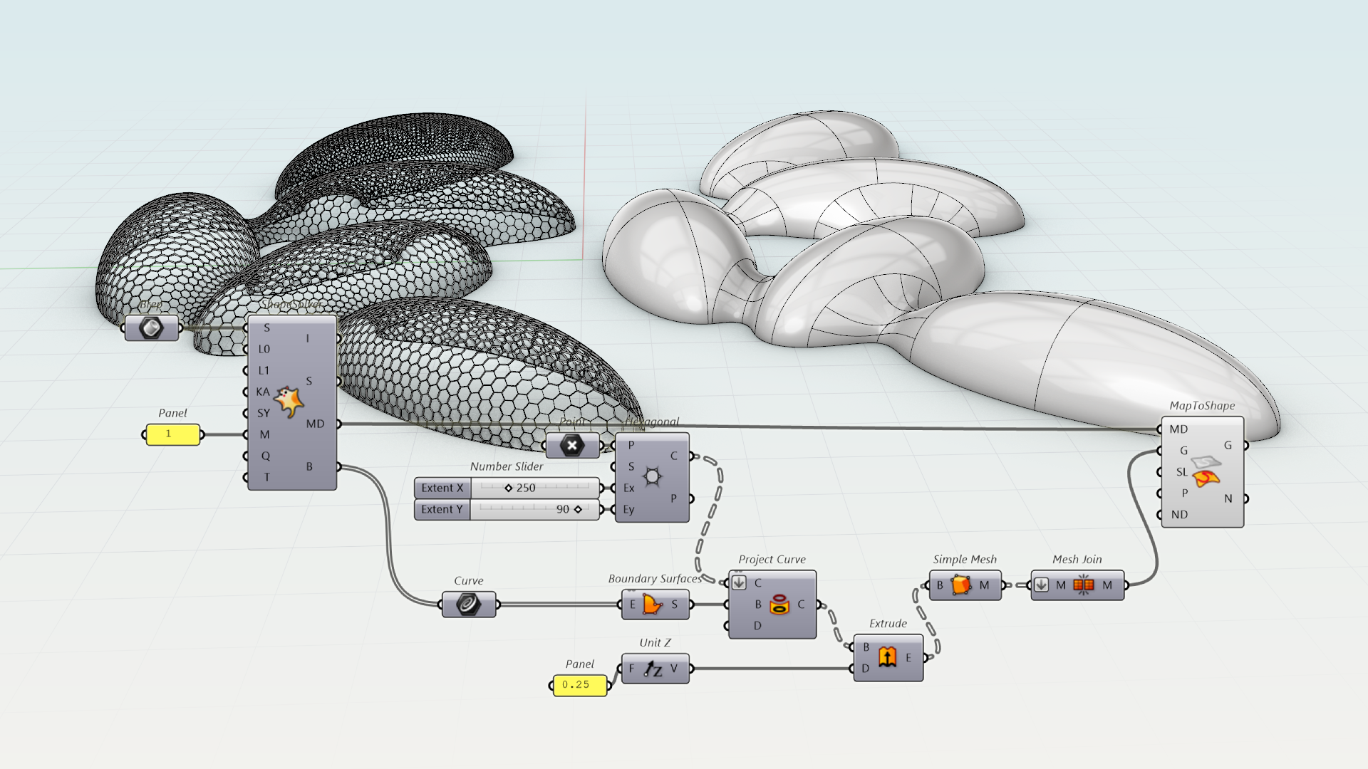
ShapeMap is a Grasshopper add-on, included with Rhino 9, that maps 2D curves or image-based textures onto a complex 3D shape, like this double-curvature polysurface, with minimal distortion. It unfolds the 3D shape into a flat one, so you can design a pattern in 2D, and then wraps the pattern back onto the original shape.
In this tutorial, you will learn the basic workflow of ShapeMap and how to use its main components, such as ShapeSolver and MapToShape, to construct a parametric hexagonal grid, representing the steel structure that wraps around the envelope.
What you'll learn
- Unfold a double-curvature polysurface into a flat shape with the
 ShapeSolver
component.
- Design a 2D hexagonal pattern on the unfolded shape with the
 Hexagonal
and
 Project Curve
components.
- Map the flat pattern back onto the 3D envelope with the
 MapToShape
component.
- Turn the pattern lines into 3D structural members with the
 Extrude
and
 Simple Mesh
components.
Prerequisites: Rhino 9, basic Grasshopper knowledge (placing components, wiring parameters).
Getting Started
- Download the latest Rhino 9 for Windows or Mac.
- Download and open ShapeMap_Architects.3dm in Rhino 9.
-
Run
the
 Grasshopper
command and start a new definition.
Load and Unfold the Shape
ShapeSolver flattens the 3D shape into a 2D shape with as little distortion as possible, and stores the relationship between the two as map data.
- Double-click the canvas, search for Brep, and place a
 Brep
parameter.
- Right-click the Brep parameter, choose
Set one Brep, and select the polysurface in the Rhino viewport. - Search for ShapeSolver in the Transform tab and place a ShapeSolver
component on the canvas. Connect the Brep parameter to its
S(Shape) input. - Right-click the
L0(Shape Line) input and selectSet one line. Then select two points in the viewport to create the base line. - Then right-click the
L1(Target Line) input and do the same, to create the target line that positions the unfolded result. - Connect a
 Panel
with the value 2 to the
M(Method) input. This sets the unfolding method toARAP(0 isLSCM, 1 isABF++). - Search for Boundary Surfaces and place a
 Boundary Surfaces
component. Connect the
B(Border) output of ShapeSolver to itsEinput. The flattened shape appears as a planar surface next to the 3D model.
// and press
it’ll place a Panel
component on the Canvas.Design the Pattern
Now that the shape is flat, you can draw the pattern in 2D, where it is easy to control.
- Continue with your file or SM_Archi_0.gh in Grasshopper.
- Place a Hexagonal
component and a
 Point
parameter. Connect the Point to the
Pinput of Hexagonal. - Right-click the Point parameter, select
Set one Point. Select a location in the Rhino viewport near the lower-left corner of the unfolded shape. This is where the grid starts. - Connect two Panel
to the
Ex(Extent X) andEy(Extent Y) inputs of Hexagonal, and set them to 100 and 45. These are the number of cells in the X and Y directions, enough to cover the whole unfolded shape. - Place a Project Curve
component. Connect the
C(Cells) output of Hexagonal to itsC(Curve) input, and theS(Surfaces) output of Boundary Surfaces to itsB(Brep) input. Only the parts of the grid that fall on the unfolded shape are kept. - Turn off the preview of the components you don’t need to see, so only the pattern on the unfolded shape is displayed.
 Number Slider
for the Extent inputs of the Hexagonal component. Define a range of values so you can interactively increase or decrease the size of your grid without having to edit the Panel each time.
Map the Pattern onto the Shape
MapToShape uses the map data from ShapeSolver to wrap the flat pattern back onto the 3D shape.
- Continue with your file or SM_Archi_1.gh in Grasshopper.
- Place a MapToShape
component found in the Transform tab. Connect the
MD(Map Data) output of ShapeSolver
to its MDinput. - Connect the
C(Curve) output of Project Curve
to the G(Geometry) input of MapToShape. The component turns red, because the data structures don’t match yet. - Right-click the
Ginput of MapToShape and chooseFlatten. The hexagonal curves are mapped onto the 3D shape.
Build the 3D Structure
The mapped curves are only lines. To get structural members with a height, extrude the flat pattern first, and then map the result.
- Continue with your file or SM_Archi_2.gh in Grasshopper.
- Place an
 Explode
component and connect the
C(Curve) output of Project Curve
to its C(Curve) input. Each hexagon is split into its individual segments. - Place a removeDuplicateLines component found in the Kangaroo2 tab. Connect the
S(Segments) output of Explode to itsLinput. Right-click theL(Lines) input and chooseFlatten. Neighboring hexagons share edges, so this removes the overlapping segments. - Place an Extrude
component, a
 Unit Z
component, and a Panel
. Set the Panel to 0.5, and connect it to the
F(Factor) input of Unit Z. Connect theV(Unit vector) output of Unit Z to theD(Direction) input of Extrude. - Connect the
Q(unique lines) output of removeDuplicateLines to theBinput of Extrude. Each line becomes a vertical strip. - Place a Simple Mesh
component and connect the
E(Extrusion) output of Extrude to itsB(Brep) input. - Connect the
M(Mesh) output of Simple Mesh to theG(Geometry) input of MapToShape
, replacing the connection from Project Curve. The hexagonal structural members now wrap around the 3D envelope, with their height following the surface normal.
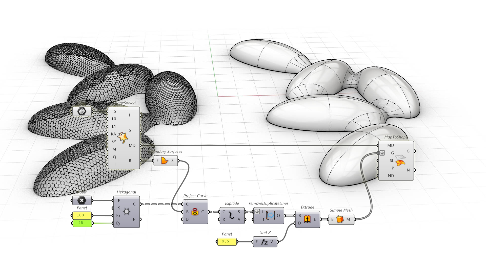
Ex and Ey values, move the Point, or change the extrusion height, and the structure updates on the envelope. Try it on your own shape too.
