Using a Bitmap Scan in the Background

The Picture command is used to bring one or more reference images into a Rhino model.

A ‘picture’ is a planar surface with the digital image added to the plane’s material as a texture.
You choose the image that the Picture will display.
Pictures can be moved, rotated, scaled and otherwise manipulated just like any Rhino object. This makes them very convenient to get them scaled and located exactly where they are needed.

In this exercise we’ll bring in two simple sketches with different views of the same object, and we’ll place the planes so that their locations and scales make sense with one another and with the scale of the object. Along the way we’ll look at some different ways to manage Pictures using layers and materials, and we’ll look at some curve and surfacing tools as well.

To begin, open the file Handset.3dm. This file does not have any objects in it yet, only some layers set up to save us a bit of time organizing. There is a layer for the Pictures - make that the current layer.

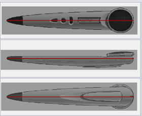
We will begin by taking scanned sketches and placing them in three different viewports. The three hand-drawn images need to be placed in their respective viewports and scaled appropriately so that they match each other.

Exercise 8-1 Handset

Open and prepare the model

Open the model Handset.3dm.
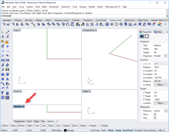
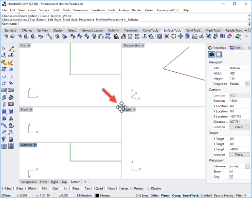
Drag the center of the Viewports to increase the height of the Top and Perspective viewports to 2/3 the size of the graphics area.
Make the **Front **viewport current.
From the **View **menu, under **Viewport Layout **click Split horizontally.
This will make a second **Front **viewport.
Highlight the lower **Front **viewport. From the **View **menu, under **Set View **click Bottom view.
Re-align the views if necessary.
In Rhino Options, on the View page, in the** Viewport properties **section, check the Linked viewports option.
This allows the viewports to stay aligned with each other when zooming and panning.

Place background bitmaps

We will begin by making reference geometry to help in placing the bitmaps.

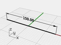
Draw a horizontal Line, from both sides of the origin of the Top viewport, 150 mm long.
Toggle the grid off in the viewports that you are using to place the bitmaps by pressing the F7 key.
This will make it much easier to see the bitmap.
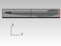
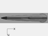
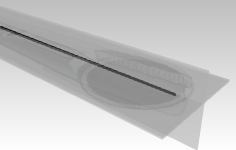
In the Front viewport, from the **Surface **menu, under **Plane **click Picture command.
In the **Open Bitmap **dialog, select the HandsetElevation.bmp.
In the **Front **viewport, using the End osnap, pick the left end of the reference line and then the right end of the reference line.
Highlight the picture in the **Front **viewport. Double click the viewport title to maximize the view.

Scale and position the background bitmaps

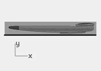
The bitmap was placed but the scale is not correct. You will orient and scale the image at the same time.

From the **Transform **menu, under Orient, click 2 Points.
On the command-line, set the **Orient **options **Copy=No **and Scale=3D.
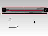
At the **Reference point 1 **prompt, pick at the left end of the image, but do not pick at the end of the Picture surface. (Use the ALT key to temporarily disable the Osnaps.)
At the **Reference point 2 **prompt, pick at the right end of the image. but do not pick at the end of the Picture surface. (Use the ALT key to temporarily disable the Osnaps.)
At the **Target point 1 **and **Target point 2 **snap to the end points of the 150 mm line that correspond the reference points.
Change to the Bottom viewport.
Use the same technique to place and align the HandsetBottom.bmp in the Bottom viewport.
Repeat these steps for placement and orientation of the **HandsetTop.bmp **in the Top viewport.
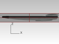
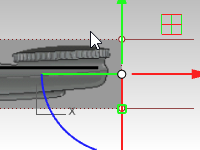
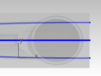
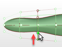
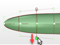
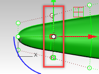
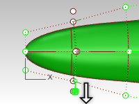
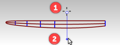
Using the Gumball, move the Top Picture object by a small amount in the Z direction (blue arrow) until the top image is visible.
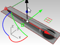
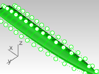
Use the Control points on the edge of the Picture object to adjust the size until all 3 images look appropriately aligned in the **Perspective **viewport.

Managing the images

Now that the images are placed and scaled, you can start using them to reference while drawing curves.

There may be times when you want to hide the objects, you probably will want to lock them so they cannot be moved by mistake. To avoid their being selectable, you can lock the layer.

You may also want to make the Pictures transparent since they may occlude objects in the 3D space.

In short you may want some tools to manage the things - this becomes more important in more complex models with multiple picture objects.

Layers

We placed the image planes on their own layer called Bitmaps. This layer can be turned on and off to show and hide the objects that are on that layer. The layer can also be locked to keep the objects from being selected.

Snapping to the Picture

One more step can make modeling a little easier as well. You probably do not want object snaps to snap to the Picture objects. You can control this, assuming the layer is locked, using the **SnapToLocked **command.

By disabling this command, and locking the layer the Pictures are on, you will not snap to these Picture objects. This command also has a Toggle option and it is nestable - you can use this command any time to set snapping behavior for locked objects, even inside another command.

You can make this command easy to access by assigning this macro to a Keyboard shortcut In Options.

'_Snaptolocked _toggle

Transparency

If the colors are too saturated or you want to dim the reference images or make them transparent to a degree in order to see other geometry, you can make them semi-transparent.

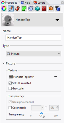
To do this highlight the Picture.

On the **Properties **panel, on the Materials page, in the Transparency area, drag the slider to 60-70 percent or a setting that looks appropriate on your system. Set transparency so that the image is just clear enough to trace against but not completely occluding the rest of the scene.

Drawing the curves with InterpCrv

Keep in mind the previous discussion on layer visibility, locking and other ‘management’ tools and making changes as needed as we go. Next you will start by drawing the curves.

You will be creating curves to define the basic shape of the case, but not any of the details or other features. For additional practice, work to finish the model beyond the details provided in this text.

There are two curve commands that are obvious choices to make the curves.

The first is the **InterpCrv **command, while the second is the with the **Curve **command.

While the more obvious choice for tracing is typically the **InterpCrv **command since you can pick exactly, along the pixels in the images, where you want the curve to fall. It is not always the best tool.

Drawing the curves with Curve

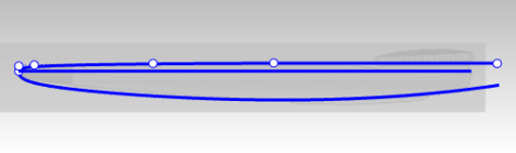
Another way to draw these curves is to use the command Curve, also called the Control Points curve.

Place the curve control points approximately where they should to be located to define the shape and use approximately the correct quantity of control points.
Next edit the curve to further refine the shape.
To refine the shape, add or remove control points as required.

With this method, creating the curves can accurately match the image with fewer control points and cleaner curves.

Authorized Rhino Trainer Gary Dawson, of Gary Dawson Designs, covers this concept in this video:
Next you will draw four curves in order to define the required shape:

one in the **Bottom **view, representing one half of the shape in that view
three in the **Front **viewport: top edge or outline, the bottom edge and the curve in the middle which is the parting line curve.

The most useful tool for tracing free-form curves is a control point curve or the **Curve **command. Here are a few pointers for the next part of this exercise.

Place the fewest number of points that will accurately describe the curve.
Avoid the trap of trying to be 100% accurate with every point placement.
With some experience you will be able to place about the correct number of points in about the correct places.
Then use control point editing to adjust the curve into its final shape.

In this example, the 2‑D curves can all be drawn quite accurately with a degree‑3 curve using five or at most six control points.

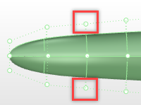
Remember to pay attention to the placement of the second points of the curves to maintain tangency across the pointed end of the object.

Drawing the Bottom view curve

From the **Curve **menu, from Free-Form, click the **Control Points **command.
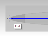
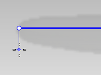
In the **Bottom **viewport, set the start of the curve by snapping to the end of the reference line
All the curves will start by snapping to this same curve end point.
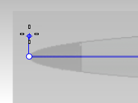
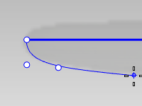
Click the second point directly above the end point in the CPlane Y direction using Ortho or SmartTrack. This will ensure that a mirrored copy of this curve will have good continuity across the end point.
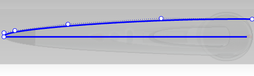
Place four more points - six total should be plenty, five may be enough.
Overshoot the open end of the shape - we’ll be trimming that off anyway shortly.
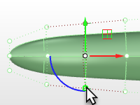
Adjust the points to make the curve match the image closely - notice that with so few points, the simple shape is very easy to match up. Gumball is a great tool for making these adjustments.
Use the **Mirror **command to mirror the curve over the reference line.

Tips for Tracing Reference Images:

Generally areas with more curvature change will have more closely spaced points.
Make sure that any adjustments to the second point from the tip of the shape is constrained to the Y axis direction.
This will ensure that the curve tangent direction stays aligned to the Y axis.

Drawing the Front view curves

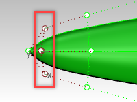
Set the second point directly below the end using Ortho- again, this sets the tangent direction to be parallel to the CPlane Y axis.
Place the rest of the points. Don’t worry too much about how far down the point falls, They will be adjusted later.
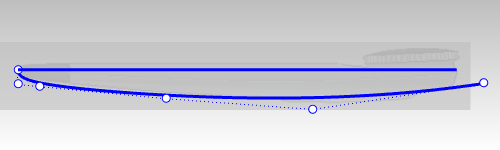
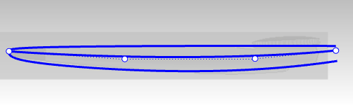
The top edge - this is almost exactly the same process as the previous curve.
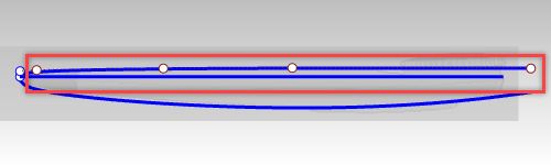
To make sure the points along the straight part of the outline are lined up horizontally, use **SetPt **command after curve has been created.
Window select the points on the top of the curve, but avoid the first two points on the curve.
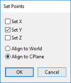
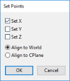
On the **Transform **menu, click Set X Y Z Coordiante.
Click **Set Y **for the CPlane Y coordinates only using the Align to Cplane option. Click the Ok.
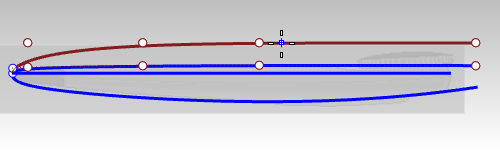
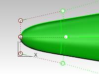
At the Location for Points, pick the second point on the curve.

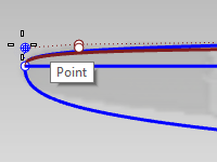
The points along the straight part of the outline are truly lined up horizontally

The parting line curve

Draw one more control point curve along the faint parting line in the image, between the top and bottom curves. This one only needs four points.

Option: Draw a line curve by picking two points. Use the **Rebuild **command to rebuild the curve as a *degree-3 *curve with four control points. Control point edit as required to match the parting line.
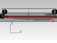
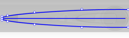
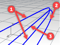
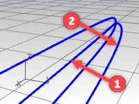
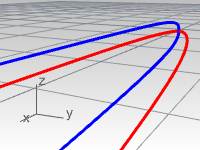
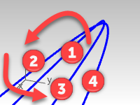
You should now have four curves. Turn off the reference layers to hide the pictures in order to see the curves clearly. (1) Curves in **Front **view, (2) Curve in **Bottom **view, (3) Parting line curve in **Front **view

Make a 3d curve from 2d curves

All of these curves are planar and two of them actually represent 2d views of the same 3d curve. The curve you drew in the **Bottom **view is a trace of the same part of the object as the parting line curve we drew in the elevation view. You need to build the curves that represent where the curves fall in 3-D space.

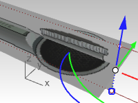
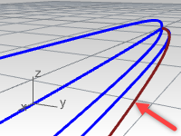
In the Perspective viewport, select the parting line curve (1) and the outline curve that you created in the **Bottom **viewport (2).
Use the Crv2View command (Curve menu: Curve From 2 Views) to create a curve based on the selected curves.
A 3‑D curve is created.
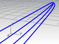
Hide or Lock the two original curves.
Now there are three curves.
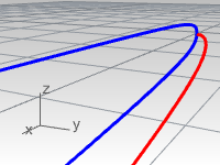
Mirror the 3‑D curve for the other side.
The macros ! Mirror 0 1,0,0 and ! Mirror 0 0,1,0 are very useful for accomplishing this quickly if they are assigned to a command alias and if the geometry is symmetrical about the x- or y-axis.

Trim the curves

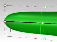
Before making the surface from the curves, trim these curves in the **Front **viewport. They were drawn to arbitrary lengths. This will insure the appropriate length and shape. It will be much easier to make a clean surface if they are all cut to the same line.

Turn **On **the **Bitmap **layer. The Pictures need to be visible but the layers should be locked.
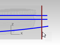
In the **Front **viewport start the **Trim **command and pick the **Line **option. Set the line vertically between the ends of the shortest curve and the end of the object in the image. Then Enter.
In the **Front **view make a right to left ‘crossing’ selection on the curve ends

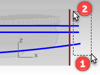
If the ends of the curves in the middle are not trimmed off, make sure the **Trim **command-line option for **ApparentIntersections **is set to **Yes **and then select the same curve ends once again.

Building the surface

Often there is more than one surfacing tool that will do the job - you will see a couple surface options and decide on the one what works best.

Start the **Loft **command and then select the curves in order. Make sure the Loft dialog is set to create a closed loft.

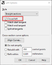
If the dialog is also set for ‘Do not simplify’ the preview of the lofted surface will show badly skewed isocurves. This is a consequence of the curves being very different in structure.
In particular the 3-D curves generated by **Crv2View **are much more complex than the curves were originally drew and these are not mixing well with the other curves in the loft.
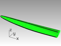
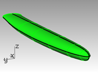
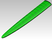
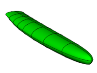
Loft the faired curves with the Closed loft option checked.
Notice the quality of the surface and how few isocurves there are.
A closed loft will have a seam.

Loft with the Rebuild option

One way to solve this is to rebuild and fair the 3d curves to a simple structure that matches the other curves, which are simpler curves. This is fine and should work- but it may be somewhat time consuming.

There is a short cut that produces a good surface and is quite efficient.

You can make a very evenly distributed smooth surface and easily adjust its points to clean up where it may not be place well, if in the Loft command you rebuild the input curves before creating the loft.

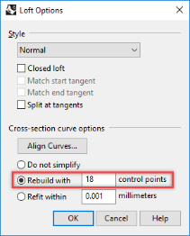
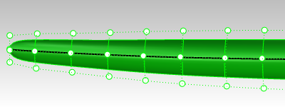
Change the setting in Loft from ‘Do not simplify’ to ‘Rebuild with’ and set the point count to 18.

You will see the isocurves even themselves out nicely immediately in the preview. With this option, the input curves are rebuilt behind the scenes. Rhino makes sure that they all have exactly the same uniform structure (degree, point count and distribution of control points.)

The result is pretty good, but not right at the end, where curvature changes rapidly

Undo until the previous Loft
Mirror the 3‑D curve for the other side.
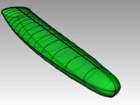
Loft the curves, using the Rebuild option to 18 points.

The isocurves all true up and everything looks clean, but if you look at the tip, it falls away from the input curves.
The Rebuild option does not sample more in areas of high curvature but just divides the curves up evenly.
The result is pretty good, but not right at the end, where curvature changes rapidly.

Clean up the lofted surface

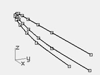
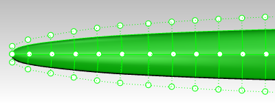
Hide the background bitmaps and set the viewport to wireframe.
Turn on surface points.
In the Top or Bottom viewport, move points on one side of the surface in the y-direction to get the surface to match.
A few points moved should do it.
Now, how do we get the other side exactly the same?
Undo all the prior moves. Next instead of moving the points, select opposite pairs of points and scale in the Y direction only using the Gumball.
**Gumball **automatically uses the middle point between the pair of selected points as the origin of the scale. Turn Ortho on to keep the scale axis true to Y axis.
Use **SetPt **in the **Bottom **view to adjust the second row of control points. This will improve the location where the curvature is changing rapidly.

In the **Bottom **view, adjust the last two or three rings of points to make the surface match the curves there.

Since the object is symmetrical in this view, it is convenient to select pairs of opposite points. Then use the **Gumball **scale handles to scale the points towards and away from each other **across **the Gumball center.

Use the **DragStrength **command to modulate the amount of scaling - this allows fine tuning with relatively large mouse movements scaling only a little.
In the side view, things are not symmetrical so move individual points.

Network surface option

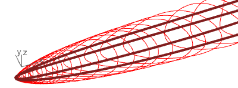
Another possibility is to create some additional curves and use the NetworkSrf command to build the surface - this command requires at least one curve in the direction ‘around’ this set of curves. The CSec command creates cross-section curves through profile curves.

Hide or delete the lofted surface.
Start the CSec command (Curve menu > Cross section profiles).
Select the curves in order as if lofting them, make sure the Closed option is Yes, press Enter when done.
For the Start cross-section line, in Front viewport, pick a point on either side of the four curves.
For the End of cross-section line, use Ortho, and pick a point on the other side of the four curves.
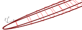
Continue this process until you have 6 to 10 cross-section curves, evenly spaced along the four curves.
Make sure to add one section snapping to the endpoints at the open end of the set of curves.
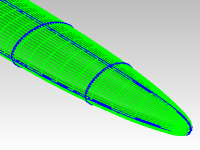
Notice in Perspective, that the result is a smooth curve interpolating between the ends of the curves. The command will keep running so you can set multiple lines in the **Front **viewport to create the smooth cross section curves. The command calculates the points of intersection of the planes represented by the lines you specify in the viewport and then interpolates a curve through those points.
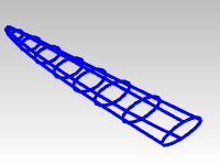
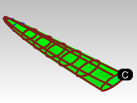
Window select the section curves and the original long curves.
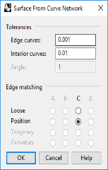
Start the NetworkSrf command (Surface menu > Curve Network) to make the surface.

On your own

Using the reference images, add additional details to the handset design.