Understanding curves continuity

This part of the course starts with a review of few concepts and techniques related to NURBS curves that will simplify the learning process during the rest of the class. Curve building techniques have a significant effect on the surfaces that you build from them.

Curve degree

The degree of a curve refers to the highest degree polynomial in the equation for the curve. In practice, it relates to the extent of the influence a single control point has over the length of the curve.

For higher degree curves, a control point has less local influence and a more broad influence over the entire length of the curve. It also has higher internal continuity.

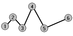
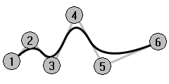
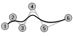
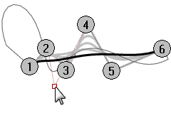
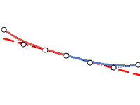
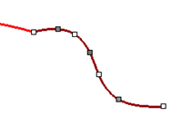
In the example below, the five curves have their control points at the same six points. Each curve has a different degree. The degree can be set with the Curve command, Degree option.

Exercise 4-1 Observe curve degree

Open the model Curve Degree.3dm.
Use the Curve command (Curve menu: Free-Form > Control Points) with Degree set to 1, using the Point object snap to snap to each of the points.
Repeat the Curve command with Degree set to 2.
Repeat the Curve command with Degree set to 3.
Repeat the Curve command with Degree set to 4.
Repeat the Curve command with Degree set to 5.

Analyze the curvature of a curve

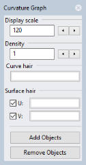
Use the CurvatureGraph command (Analyze menu: Curve > Curvature Graph On) to turn on the curvature graph for one of the curves.
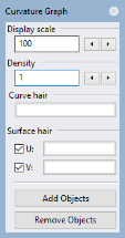
Set the Display scale to a number that shows the graph as in the illustration. A number between 110-120 should work well.
The graph indicates the curvature on the curve. This is the inverse of the radius of curvature. The smaller the radius of curvature at any point on the curve, the larger the amount of curvature.
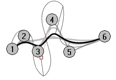
Turn on the control points for the curve you have graphed and view the curvature graph as you drag some control points.
Note the change in the curvature hairs as you move points.
Repeat this process for each of the curves.
You can use the Curvature Graph dialog box buttons to remove or add objects from the graph display.

Note

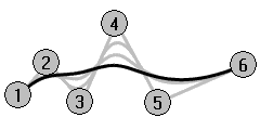
Degree 1 curves have no curvature and no graph displays.
Degree 2 curves are internally continuous for tangency. The steps in the graph indicate this condition. Note that only the graph is stepped not the curve.
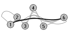
Degree 3 curves have continuous curvature. The graph will not show steps but may show hard peaks and valleys. Again, the curve is not kinked at these places. The graph shows an abrupt but not discontinuous change in curvature.
In higher degree curves, higher levels of continuity are possible.
For example, a Degree 4 curve is continuous in the rate of change of curvature. The graph does not show any hard peaks.
A Degree 5 curve is continuous in the rate of change of the rate of change of curvature. The graph does not show any particular features for higher degree curves but it will tend to be smooth.
Changing the degree of the curve to a higher degree with the ChangeDegree command with Deformable=No will not improve the internal continuity, but lowering the degree will adversely affect the continuity.
Rebuilding a curve with the Rebuild command will change the internal continuity.

Curve and surface continuity

Since creating a good surface so often depends upon the quality and continuity of the input curves, it is worthwhile clarifying the concept of continuity among curves.

For most curve building and surface building purposes we can talk about four useful levels of continuity:

Not continuous

The curves or surfaces do not meet at their end points or edges. Where there is no continuity, the objects cannot be joined.

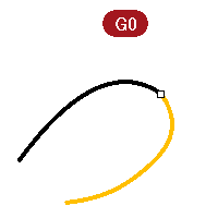
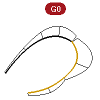
Positional continuity (G0)

Curves meet at their end points, surfaces meet at their edges.

Positional continuity means that there is a kink at the point where two curves meet. The curves can be joined in Rhino into a single curve but there will be a kink and the curve can still be exploded into at least two sub-curves.

Similarly two surfaces may meet along a common edge but will show a kink or seam, a hard line between the surfaces. For practical purposes, only the endpoints of a curve or the last rows of points along the edges of two untrimmed surfaces need to match to determine G0 continuity.

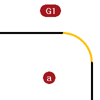
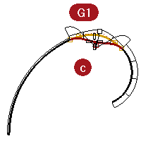
Tangency continuity (G1)

Curves or surfaces meet and the directions of the tangents at the endpoints or edges is the same. You should not see a crease or a sharp edge.

Tangency is the direction of a curve at any particular point along the curve

Where two curves meet at their endpoints the tangency condition between them is determined by the direction in which the curves are each heading exactly at their endpoints. If the directions are collinear, then the curves are considered tangent. There is no hard corner or kink where the two curves meet. This tangency direction is controlled by the direction of the line between the end control point and the next control point on a curve.

In order for two curves to be tangent to one another, their endpoints must be coincident (G0) and the second control point on each curve must lie on a line passing through the curve endpoints. A total of four control points, two from each curve, must lie on this imaginary line.

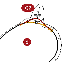
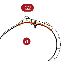
Curvature continuity (G2)

Curves or surfaces meet, their tangent directions are the same and the radius of curvature is the same for each at the endpoint.

Curvature Continuity includes the above G0 and G1 conditions and adds the further requirement that the radius of curvature be the same at the common endpoints of the two curves. Curvature continuity is the smoothest condition over which the user has any direct control, although smoother relationships are possible.

For example, G3 continuity means that not only are the conditions for G2 continuity met, but also that the rate of change of the curvature is the same on both curves or surfaces at the common endpoints or edges.

G4 means that the rate of change of the rate of change of the curvature is the same for both curves where they meet. This is the smoothest type of join. Rhino has tools to build such curves and surfaces, but fewer tools for checking and verifying such continuity than for G0-G2.

G5+ has no visible evidence of more continuity.

Curve continuity and curvature graph

Rhino has two analysis commands that will help illustrate the difference between curvature and tangency. In the following exercise, we will use the CurvatureGraph and the Curvature commands to gain a better understanding of tangent and curvature continuity.

Show continuity with a curvature graph

Open the model Curvature_Tangency.3dm.
There are five sets of curves, divided into three groups.
One group has positional (G0) continuity at their common ends.

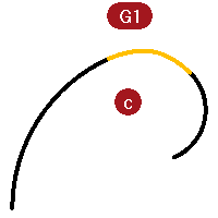
Group (a-c) has tangency (G1) continuity at their common ends.

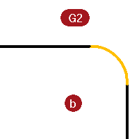
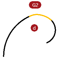
Group (b- d) has curvature (G2) continuity at their common endpoints.
Press Ctrl + A to select all of the curves.
Turn on the Curvature Graph (Analyze menu: Curve > Curvature Graph On) for the curves.
Set the Display scale in the floating dialog box to 100.
Change the scale if you cannot see the curvature hair.
The depth of the graph at this setting shows, in model units, the amount of curvature in the curve.
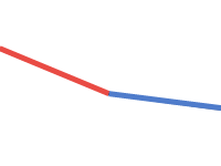
Notice the top sets of curves (a-b).
These two lines have a curve between them.
Lines have no curvature and therefore do not show a curvature graph.
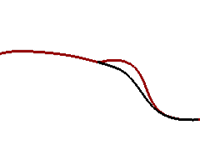
The image below shows what happens when the curvature is not continuous. The sudden jump in the curvature graph indicates a discontinuity in curvature.
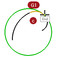
The G1 middle curve is an arc. It shows a constant curvature graph as expected because the curvature of an arc never changes, just as the radius never changes.

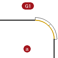
Nevertheless the line-arc-line is smoothly connected. The arc picks up the exact direction of one line and then the next line takes off at the exact direction of the arc at its end.
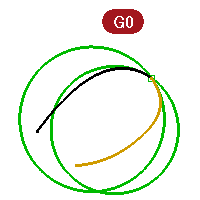
On the other hand, the G2 curves (b) again show no curvature on the lines, but the curve joining the two lines is different from the G1 case. This curve shows a graph that starts out at zero, it comes to a point at the end of the curve, increases rapidly but smoothly, and then tails off again to zero at the other end where it meets the other straight line segment. It is not a constant curvature curve and thus not a constant radius curve. The graph does not have a sudden jump in the curvature graph; it goes smoothly from zero to its maximum.
For the G2 middle curve, the graph ramps up from zero to some maximum height along a curve and then slopes back to zero, matching the zero curvature again on the other straight line.

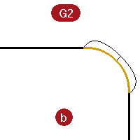
Thus, there is no discontinuity in curvature from the end of the straight line to end of the curve. The curve starts and ends at zero curvature just like the lines have. So, the G2 case not only is the direction of the curves the same at the endpoints, but the curvature is the same there as well. There is no jump in curvature, and the curves are considered G2 or curvature continuous.
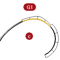
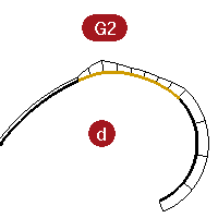
Look at the c and d curves.
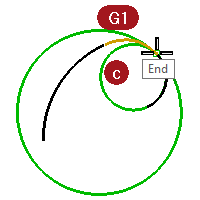
These are also G1 and G2 but are not straight lines so the graph shows up on all of the curves.
Again, the G1 set shows a step up or down in the graph at the common endpoints of the curves. This time the curve is not a constant arc. The graph shows that it increases in curvature out towards the middle.
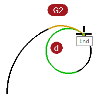
On G2 curves, the graph for the middle curve shows the same height as the adjacent curves at the common endpoints. There are no abrupt steps in the graph.
The outer curve on the graph from one curve stays connected to the graph of the adjacent curve.

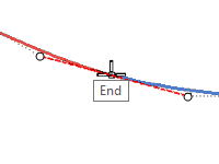
Show continuity with a curvature circle

Start the Curvature command (Analyze menu: Curvature circle) and select the middle curve in set c.
The curvature circle that appears on the curve indicates the radius of curvature at that location. The curvature circle results from the center and radius measured at that point on the curve.
Drag the curvature circle along the curve.
Notice that where the circle is the smallest, the graph shows the largest amount of curvature. The curvature is the inverse of the radius at any point.
On the command-line, click the MarkCurvature option.
Slide the curvature circle, snap to an endpoint of the curve, and click to place a curvature circle.
Stop the command and restart it for the other curve sharing the endpoint just picked.
Place a circle on this endpoint as well.
The two circles have greatly different radii. Again, this indicates a discontinuity in curvature. These curves are G1/tangent only, so the curvature at the tangent meeting point is different for the two curves, and that is where the curvature graph would take a jump.
Repeat the same procedure to get circles at the ends of the curves in set d.
Notice that this time the circles from each curve at the common endpoint are the same radius. These curves are curvature continuous.
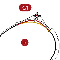
Turn on the control points for the middle curves in c and d.
Select the middle control point on either curve and move it around.
Notice that while the curvature graph changes greatly, the continuity at each end with the adjacent curves is not affected.
The G1 curve graphs stay stepped, though, the size of the step changes.

The G2 curve graphs stay connected, although there is a peak that forms there.
Look at the graphs for the G0 curves.
Notice that there is a gap in the graph. This indicates that there is only G0 or positional continuity.
The curvature circles, on the common endpoints of these two curves, are not only different radii, but they are also not tangent; they cross each other. There is a discontinuity in direction at the ends.

Exercise 4-2 Examine geometric continuity

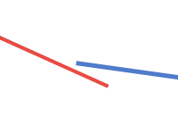
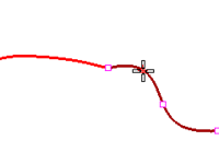
Open the model Curve Continuity.3dm.
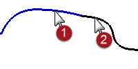
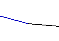
The two curves are clearly not tangent.
Verify this with the continuity checking **GCon **command .
Start the GCon command (Analyze menu: Curve > Geometric Continuity).
Click near the common ends (1 and 2) of each curve.
Rhino displays a message on the command-line indicating the curves are out of tolerance. The endpoints of the two curves are not close enough to each other to be considered the same.
Curve end difference = 0.030 millimeters
Radius of curvature difference = 126.531 millimeters
Curvature direction difference in degrees = 10.277
Tangent difference in degrees = 10.277
Curve ends are out of tolerance.
Often, imported curves are often out of tolerance and need repair for accurate modeling.

Make curves have position continuity

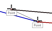
Turn on the control points for both curves and zoom in on the common ends.
Turn on the Point object snap and drag one of the endpoints onto the other.
Repeat the **GCon **command.
The command-line message is different now:
Curve end difference = 0.000 millimeters
Radius of curvature difference = 126.771 millimeters
Curvature direction difference in degrees = 10.307
Tangent difference in degrees = 10.307
Curves are G0.
Undo the previous operation.

Change curves to position continuity

The Match command provides a tool for moving the curve endpoints automatically.

Start the Match command (Curve menu: Curve Edit Tools > Match).
Pick near the common end of one of the curves.
Pick near the common end of the other curve.
By default, the curve you pick first will be the one that is modified to match the other curve.
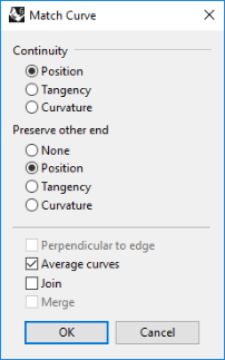
To make both curves change to an average of the two, in the Match Curve dialog box, check the Average Curves option.
In the Match Curve dialog box, for Continuity, check the Position option, for Preserve other end, check the Position option, check the Average Curves option.
Repeat the GCon command.
The command-line message indicates:
Curve end difference = 0.000 millimeters
Radius of curvature difference = 126.708 millimeters
Curvature direction difference in degrees = 10.265
Tangent difference in degrees = 10.265
Curves are G0.

Set up aliases

Along and Between are one-time object snaps that are available in the Tools menu under Object snaps. They can be used only after a command has been started and apply to only one pick.

Before we continue, we will create some aliases that will be used in the next exercises.

Exercise 4-3 Make Along and Between aliases

In the Rhino Options dialog box on the Aliases page, click the New button
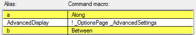
In the Alias column, type a.
In the Command macro column, type _Along.
In the Alias column type b.
In the Command macro column, type _Between.
Close the Rhino Options dialog box.

Tangent continuity

It is possible to establish a tangency (G1) condition between two curves by aligning the control points in a particular way. The endpoints at one end of the curves must be coincident and these points in addition to the next point on each curve must fall in a line with each other. This can be done automatically with the **Match **command, although it is also easy to do by moving the control points using the normal Rhino transform commands.

We will use Move, SetPt, Rotate, Zoom Target, PointsOn F10, PointsOff F11 commands and the object snaps End, Point, Along, Between and the Tab lock to move the points in various ways to achieve tangency.

Tab direction lock

The Tab direction lock locks the movement of the cursor when the Tab key is pressed. It can be used for moving objects, dragging, or curve and line creation.

To activate Tab direction lock press and release the Tab key when Rhino is asking for a location in space. The cursor will be constrained to a line between its location in space at the time the Tab key is pressed and the location in space of the last clicked point.

When the direction is locked, it can be released with another press and release of the Tab, and a new, corrected direction set with yet another Tab press.

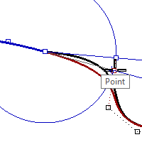
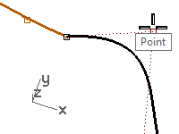
Change the continuity using Rotate and the Tab direction lock

Turn on the control points for both curves.
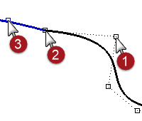
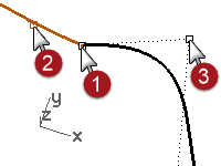
Select the control point (1) second from the end of one of the curves.
Start the Rotate command (Transform menu: Rotate).
Using the Point object snap, select the common endpoints (2) of the two curves for the Center of rotation.
For the First reference point, snap to the current location of the selected control point.
For the Second reference point, make sure the point object snap is still active.
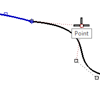
Hover the cursor, but do not click, over the second point (3) on the other curve.
While the Point object snap flag is visible on screen, indicating the cursor is locked onto the control point, press and release the Tab key.
Do not click with the mouse.
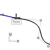
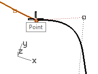
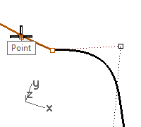
Bring the cursor back over to the other curve.
Notice that the position is constrained to a line between the center of rotation and the second point on the second curve; that is, the location of the cursor when you press the Tab key. You can now click the mouse on the side opposite the second curve.
During rotation, the Tab direction lock knows to make the line from the center and not from the first reference point.
The rotation endpoint will be exactly in line with the center of rotation and the second point on the second curve.

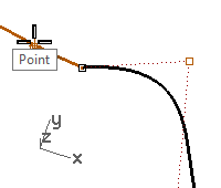
Change the continuity by adjusting control points

Use the OneLayerOn command to turn on only the 3D Curves layer.
Check the continuity of the curves with the GCon command.
Turn on the control points for both curves.
Window select the common endpoints of both curves (1).
Use the Move command (Transform menu: Move) to move the points.
For the Point to move from, snap to the same point (1).
For the Point to move to, type b and press Enter to use the Between object snap.
For the First point, snap to the second point (2) on one curve.
For the Second point, snap to the second point (3) on the other curve.
The common points are moved in-between the two second points, aligning the four points.
Check the continuity.

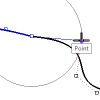
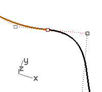
Change the continuity by adjusting control points using the Along object snap

Undo the previous operation.
Select the second point (3) on the curve on the right.
Use the Move command (Transform menu: Move) to move the point.
For the Point to move from, snap to the selected point.
For the Point to move to, type A and press Enter to use the Along object snap.
For the Start of tracking line, snap to the second point (2) on the other curve.
For the End of tracking line, snap to the common points (1).
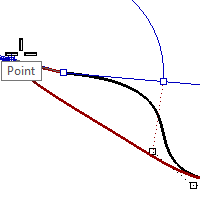
The point tracks along a line that goes through the two points, aligning the four points.
Click to place the point.
Check the continuity.

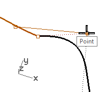
Edit the curves without changing the tangency direction

With the Tab technique, we can adjust the meeting point of the curves, or the shape of either curve near the meeting point, without losing the G1 continuity.

Window select the common endpoints or select the second point on either curve.
Turn on the Point object snap and drag the point(s) to the next one of the four critical points.
When the Point object snap flag shows on the screen, use the Tab direction lock by pressing and releasing the Tab key without releasing the mouse button.
Drag the point(s) and the tangency is maintained since the drag direction is constrained to the Tab direction lock line.
Release the left mouse button at any point to place the point(s).

Note

To maintain G1 continuity make sure that any point manipulation of the critical four points takes place along the line on which they all fall.
Once you have G1 continuity you can still edit the curves near their ends without losing continuity, using the Tab direction lock.
This technique only works after tangency has been established.

Edit the curves using Dragmode

Start the **DragMode **command, and choose ControlPolygon at the command line
Note: the cursor changes to indicate the drag mode has changed from the default CPlane based dragging.
ControlPolygon only applies to curve and surface control points.
Disable **Osnap **in the Status bar.
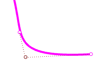
Select the second point from one end of the curve and drag it towards the end point - the dragging is constrained to the control polygon line connecting the points. This ensures that the tangent direction on the curve does not change.
Now drag the point to the left and away from the end point on the curve that is on the right.
The point is constrained to the control polygon of the third point. This control edit breaks that tangency direction of the curve.
To maintain the tangent direction of the curve, drag towards the end point a short distance first, hit **Tab **to constrain that direction and then drag away from the end point. Dragging a point with the **Tab **constrains the direction to the curve or surface normal.
Run DragMode again to switch back to CPlane drag mode.

The Dragmode Macros

Running the same drag mode option twice in a row returns drag mode to the default, so you can make a shortcut or alias for:
! _DragMode _ControlPolygon

! _DragMode _Cplane

Use these to toggle back and forth quickly between default and control polygon modes.

Go to **Options **and **Keyboard **and add the **Macro **to keys Control +F6 and Control +F7.

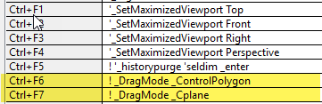
Note: You will find the macro command in the Macros.txt which is included in the Level 2 model set.

Curvature continuity

Adjusting points to establish curvature continuity is not as straightforward as for tangency. Curvature at the end of a curve is determined by the position of the last three points on the curve, and their relationships to one another are not as straightforward as it is for tangency.

To establish curvature or G2 continuity, the **Match **command is the only practical way in most cases.

Exercise 4-4 Match the curves

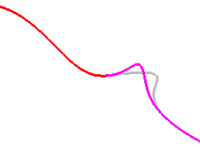
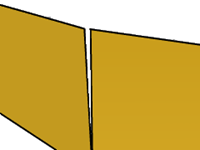
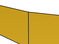
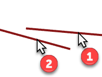
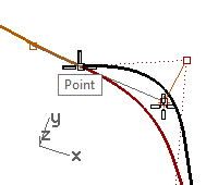
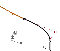
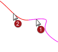
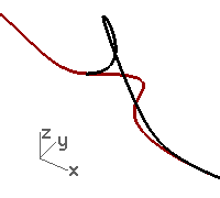
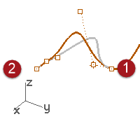
Use the Match command (Curve menu: Curve Edit Tools > Match) to match the magenta (1) curve to the red (2) curve.
Set Continuity to Curvature, Preserve other end to Curvature, and clear the Average curves option.

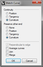
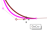
When you use Match with Curvature checked on these particular curves, the third point on the curve to be changed is constrained to a position calculated by Rhino to establish the desired continuity.

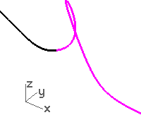
The curve being changed is significantly altered in shape.
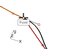
Moving the third point by hand will break the G2 continuity at the ends, though G1 will be maintained

Advanced techniques for controlling continuity

There are two additional methods to edit curves while maintaining continuity in Rhino. (1) The **EndBulge **command constrains points at the end to maintain continuity with the adjacent curve. (2) Adding knots will allow more flexibility when changing the curve’s shape.

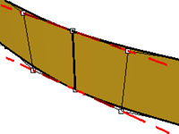
Edit the curve with end bulge

Right-click the Copy button to make a duplicate of the magenta curve and then Lock it.
Start the EndBulge command (Edit menu: Adjust End Bulge).
Select the magenta curve.
Notice that there are more points displayed than were on the original curve.
The EndBulge command adds more control points to the curve if the curve has less than the required control point count.
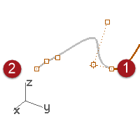
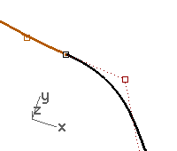
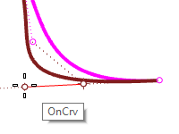
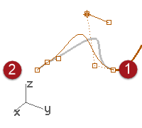
Select the third point, drag it, and click to place the point, press Enter to exit the command.
If the endpoint of the curve has G2 continuity with another curve, the G2 continuity will be preserved, because EndBulge preserves the curvature at the endpoint of the curve.

Note: Adjusting control points will work to match curvature only in the simple case of matching to a straight line.

Add a knot

Adding a knot or two to the curve will put more points near the end so that the third point can be nearer the end. Knots are added to curves and surfaces with the InsertKnot command.

Undo your previous adjustments.
Start the InsertKnot command (Edit menu: Control Points > Insert Knot).
Select the magenta curve.
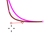
Pick a location on the curve to add a knot in between the first two knot markers.
In general, a curve or surface will tend to behave better in point editing if new knots are placed midway between existing knots, thus maintaining a uniform distribution.
Adding knots also results in added control points.

Knots and control points are not the same thing and the new control points will not be added at exactly the new knot location.
The Automatic option automatically inserts a new knot in each span exactly half way between existing knots.
If you only want to place knots in some of the spans, you should place these individually by clicking on the desired locations along the curve.
Existing knots are highlighted in white.
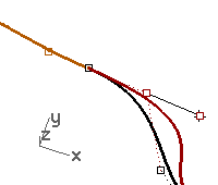
Match the curves after inserting a knot into the magenta curve.
Inserting knots closer to the end of curves will change how much Match changes the curve.