Since Rhino is a mathematically accurate NURBS modeler, it includes tools to provide accurate information about the objects.
Rhino has several tools to help you visually evaluate surface quality. In this exercise, we will use curve and surface analysis tools to help build clean, simple surfaces with good continuity.
Some models require more attention to continuity, primarily, because it will show when manufactured. For example, a blow-molded bottle will not show slight inconsistencies in the surface, but a car panel will.
Measure distance, angle, and radius
Some analysis commands provide information about location, distance, angle between lines, and radius of a curve. For example:
- Distance displays the distance between two points.
- Angle displays the angle between two lines.
- Radius displays the radius of a curve at any point along it.
- Length displays the length of a curve.
 Direction
Curves and surfaces have a direction. Many commands that use direction information display direction arrows and give you the opportunity to change (flip) the direction.
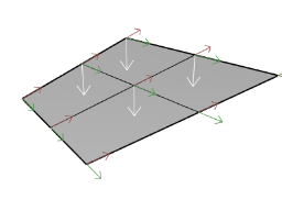
Every surface is roughly rectangular. Surfaces have three directions: u, v, and normal.
The u‑ and v‑directions are like the weave of cloth or screen. The u‑direction is indicated by the red arrow, and the v‑direction is indicated by the green arrow. The colors match the grid axis colors. The normal direction is indicated by the white arrow. You can think of u-, v-, and normal-directions as corresponding to the x, y, and z of the surface.
These directions are used when mapping textures and inserting knots.
The Dir command displays the direction of a curve or surface.
The illustration shows the curve direction arrows. If the direction has not been changed, it reflects the direction the curve was originally drawn. The arrows point from the start of the curve toward the end of the curve.
The Dir command can also change the direction of a curve.
Curve direction.
Surface normals are represented by arrows perpendicular to the surface, and the u‑ and v‑directions are indicated by arrows pointing along the surface. Closed surfaces always have the surface normals pointing to the exterior.
The Dir command can change the u‑, v‑, and normal‑directions of a surface. This direction can be important if you are applying textures to the surface.
Surface direction.
Visual surface analysis
Visual surface analysis commands let you examine surfaces to determine smoothness. These commands use NURBS surface evaluation and rendering techniques to help you visually analyze surface smoothness with false color or reflection maps so you can see the curvature and breaks in the surface.
 Curvature analysis
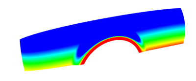
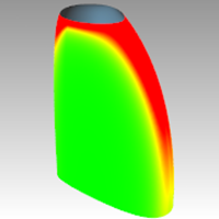
The CurvatureAnalysis command analyzes surface curvature using false color mapping. It analyzes Gaussian curvature, mean curvature, minimum radius of curvature, and maximum radius of curvature.
 Environment map
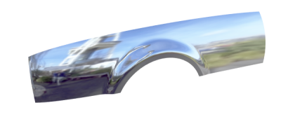
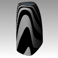
The EMap command displays a bitmap on the object so it looks like a scene is being reflected by a highly polished metal. This tool helps you find surface defects and validate your design intent.
The fluorescent tube environment map simulates tube lights shining on a reflective metal surface.
 Zebra
Zebra
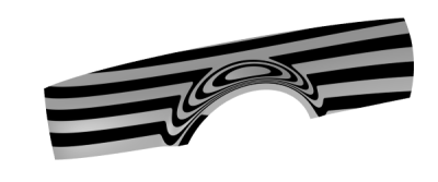
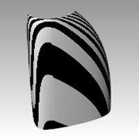
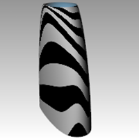
The Zebra command displays surfaces with reflected stripes. This is a way to visually check for surface defects and for tangency and curvature continuity conditions between surfaces.
 Draft angle analysis
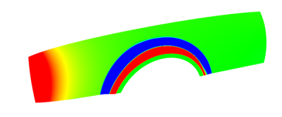
The DraftAngleAnalysis command displays the draft angle relative to the construction plane that is active when you start the command.
The pull direction for the DraftAngleAnalysis command is the z‑axis of the construction plane. It also uses false color mapping.
 Edge evaluation
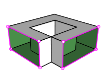
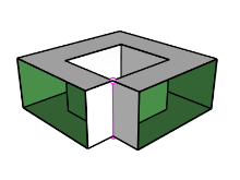
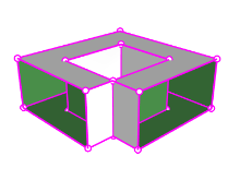
Geometry problems such as Boolean or join failures can be caused by edges on surfaces that have become broken or edges between surfaces that have been moved through point editing so they create holes. An edge is a separate object that defines the surface’s boundary.
The ShowEdges command highlights naked edges, non-manifold edges or all edges of the surface.
|  |
|  |
|  |
|
|
|
Naked edges
|
Non-manifold edges
|
All edges
|
The Properties command may tell you that a polysurface is open even though it looks closed. Some operations and export features require closed polysurfaces, and a model using closed polysurfaces is generally higher quality than one with small cracks and slivers.
When a surface is not joined to another surface, it has naked edges. Rhino provides a tool for finding the unjoined or “naked” edges. Use Properties command to examine the object details. A polysurface that has naked edges lists as an open polysurface. Use the ShowEdges command to display the unjoined edges.
Other edge tools let you split an edge, merge edges that meet end-to-end, or force surfaces with naked edges to join. You can rebuild edges based on internal tolerances. Other edge tools include:
- SplitEdge divides a surface edge at a designated point.
- MergeEdge merges edges that meet end to end.
- JoinEdge forces unjoined (naked) edges to join nearby surfaces.
- RebuildEdges redistributes edge control points based on internal tolerances.
Diagnostics
Diagnostic tools report on an object’s internal data structure and select objects that may need repair. The output from the List, Check, SelBadObjects, and Audit3dmFile commands is normally most useful to a Rhino programmer to diagnose problems with surfaces that are causing errors.
Surface analysis tutorial
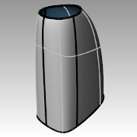
The file, Surface Analysis.3dm, has a set of curves you will recognize from the previous exercise. Our task in the current exercise is to make curves that can create cleaner, simpler surfaces with good continuity. We will make use of the CurvatureGraph, Zebra, and CurvatureAnalysis to make sure we set things up for the best results. Lastly, we will compare the surface analysis results in this file with the surface analysis results in the previous exercise.
Exercise 11-1 Surface analysis
Evaluate the curves
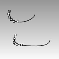
First, let us look at the curvature graphs of the top and the bottom curves. These curves have a nice enough shape, but there is room for improvement from a surfacing continuity perspective.
Open the model
- Open the file Surface Analysis.3dm.
- Select the top and bottom curves.
- Start the **CurvatureGraph **command (Analyze menu: Curve > Curvature Graph On) and set the Display scale to a value of 120.
The graph tells us that both curves are tangent continuous but have curvature discontinuities in a couple of locations.
Assuming we want the surfaces we build from these curves to have curvature continuity throughout, we will be better off modifying these curves before creating the surfaces.
If we decide ahead of time what the surface arrangement will be, that will help us understand how to draw clean new curves.
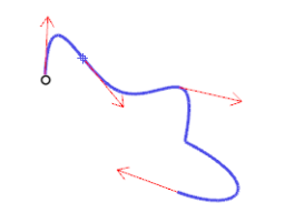
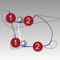
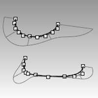
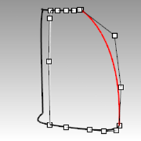
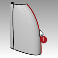
Building a surface that has consistent curvature as a single surface is good modeling practice. Looking at the bottom curve, we can see two areas that are good candidates for creating the surfaces, so we will start there. There is an area of high curvature at the front (1) and a relatively flat stretch in the middle with a rapidly increasing curvature at the handle side (2). The top curve is smoother overall, but has similar corresponding regions of curvature.
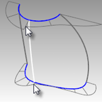
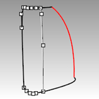
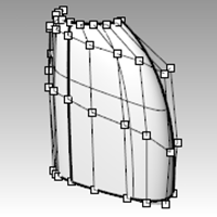
By examining the current curves, we can identify two curves to build at the top and bottom. The white vertical curve intersects the top and bottom curves at the curvature discontinuity of the top curve, which is a modified circle, and on an abrupt change in curvature on the lower curve. This intersection is where we will start and end our modified curves.
Build the modified curves
- Using the current curves as a reference, draw four new curves of degree five with six points.
The goal is to redraw the top and bottom curves in two parts each.
Keep in mind what you know about continuity, CurvatureGraph, tangent directions, and EndBulge.
Try to keep the control point locations even and progressive.
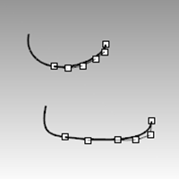
- Analyze your curves with the CurvatureGraph command.
Try to get the graph clean with minimal, abrupt changes, while at the same time match the original curve shapes as closely as possible.
They cannot be exactly the same as the originals if they are to have better continuity, but it should be possible to get close.
Make the surfaces for the bottle from edge curves
There are four, single-span, curves that define each area for the surfaces. In this part of the exercise we will use the EdgeSrf command (Surface menu: Edge curves) to create the surfaces. This command is one that uses the input curve structure to create the surface. It works best if the curves on opposite sides of the rectangle match each other. The resulting surface will be simpler.
Since we have taken care to meet this criterion, all of the vertical curves are degree 3 with four points, and the curves we just made are degree five with six points, the resulting surfaces will share this structure.
- Select four curves that define one of the surfaces.
- Start the **EdgeSrf **command (Surface menu: Edge curves).
- Repeat steps 1 and 2 for the other surface.
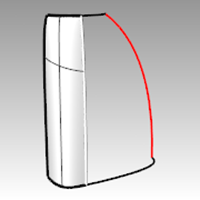
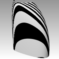
- Check the surfaces with the Zebra command.
The zebra stripes have a nice even flow but the surfaces are clearly not tangent at the vertical edge.
Match the surfaces for the bottle with MatchSrf
- Use the **MatchSrf **command (Surface menu: Surface Edit Tools > Match) to match the surfaces for Curvature.
Try matching in both directions, and with or without Average surfaces set.
In this case, the results are good no matter how the match is made, but it is worth looking at the control points on the surfaces in each case.
Matching the larger surface to the smaller one, without Average, results in a more erratic control point arrangement on the larger surface than any other combination, particularly the second row from the top. Other considerations being equal, the best choice is the surface with the most regular, even control point arrangement.
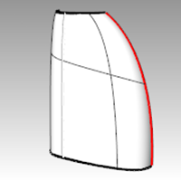
- Check the surfaces with the Zebra command.
The zebra stripes have a nice even flow with no discontinuity at the common edge.
Match the surfaces for the bottle with symmetry
In this section, we will make the other half of the bottle using the Symmetry command with Record History turned on. Symmetry mirrors curves and surfaces, makes the mirrored half tangent to the original, and with History recording active, when the original object is edited, the mirrored half updates to match the original.
- Select the larger surface.
- Use the Symmetry command (Transform menu: Symmetry) to mirror the surface across the x-axis.
- Turn Record History on.
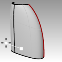
- For the Select curve end or surface edge, select the edge of the surface (1).
- For the Start of symmetry plane, type 0 and press Enter.
- For the End of symmetry plane, use Ortho to pick a point along the x-axis.
- Repeat this process for the other surface.
If you edit either original surface, the mirrored part will update to match.
- Check the surfaces with the Zebra command.
The zebra stripes have a nice even flow with no discontinuity at the common edge.
Analyze the matched surfaces
At this point, we will use the Curvature Analysis tool to evaluate the matched surfaces. This can be useful in locating areas of extreme curvature, but may force the display to ignore more subtle changes. In any case, the display on each of these simple surfaces should be very smooth and clean.
- Hide all curves to get a good view of the transitions between surfaces.
- Select all of the surfaces and turn on Curvature Analysis display (Analyze menu: Surface > Curvature Analysis).
Set the style to Gaussian, and click Auto Range. Make sure you have a fine analysis mesh for a good visual evaluation. - Click back and forth between Auto range and Max range.
Auto Range attempts to find a range of color that will ignore extremes in curvature, while Max Range will map the maximum curvature to red and the minimum to blue.
The numbers are for Curvature, which is, 1/radius.
The goal when matching is to maintain as even and gradual a curvature display as possible, while meeting the continuity requirements.
Notice the edges that have been matched appear to have a smooth color transition.
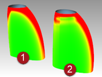
Analyze and compare different surfacing techniques
Next, we will make another surface for comparison.
- Copy the curves to one side.
- Mirror and Join the top and base curves on the x-axis.
- Mirror the vertical side curve on x-axis to make a set of curves suitable for a surface form a curve network.
- Use NetworkSrf to make a surface from these curves.
- Select the new surface and **Add **it to the Curvature Analysis display.
The denser network surface (2) has a less clean appearance in this display. The simple surfaces (1) still look cleaner at this point.
Since the color change is mapped across the entire range shown, it is important to remember that the Auto Range setting indicates a very narrow range of curvature and that the actual differences may be small even though the color change is great.